Read the entire syllabus on the course webpage
This lab should serve as a review of some CS260 topics, including:
sklearn built-in classes and methodsThis first part of this lab (a short review about object-oriented programming and custom data structures) will be done in randomly assigned pairs, but the remainder of the lab should be done individually. You may discuss concepts with fellow classmates, but you may not share or view code.
Your starting files (and submissions) will be handled using GitHub Classroom.
The recommended editor for this course is VScode, which is installed on the lab machines. You are welcome to use a different editor, as long as we can run your code on the terminal using the commands specified below.
In lab (on Tuesday), find your randomly assigned partner. If you are on the waitlist, find a random partner. For this part you should be on one machine. The person whose first name comes first alphabetically should be the “driver” (at the keyboard) and the other person should be the “navigator”. Throughout this short introduction, make sure you both understand everything!
Open the file data/colleges.txt, which lists colleges along with recent enrollment numbers. The goal is to read this file and extract the information for just the Tri-Co colleges (Bryn Mawr, Haverford, and Swarthmore). main has been provided.
Create a class Consortium whose constructor takes two parameters (in addition to self): a filename and a list of colleges to extract. The exact details of the constructor are up to you.
Create a __str__ method that will produce a printout of the colleges (and their enrollments), similar to the one below.
Create an enrollment method that will compute and print the total enrollment across the consortium.
Overall, when I run
python3 pair_exercise.pyI should obtain the following printout:
Consortium:
    BrynMawr: 1709
    Haverford: 1421
    Swarthmore: 1620

total enrollment:  4750
Note that nothing about your class should be specific to the Tri-Co.
Add both your names to the documentation and email this file to the partner who doesn’t have it, so they can add/commit/push the code to their repo as well. (We will have formal partner work in this class where you both have access to the git repo, but not for this first lab.)
Make sure to always use python3!
The data for Lab 1 is a set of handwritten digits from zip codes written on hand-addressed letters. The datasets is separated into “train” and “test”, and is available here:
/home/smathieson/Public/cs360/zip/zip.train
/home/smathieson/Public/cs360/zip/zip.test
If you would like to work on your own machine you can copy the data to a folder of your choice using scp (secure copy):
scp smathieson@cook.cs.haverford.edu:/home/smathieson/Public/cs360/zip/zip.train ~/Desktop/zip.trainJust make sure not to add/commit/push the data to your github repo! Also note that we do not have the bandwidth to debug issues on your own machine. Please use the lab machines if your machine is not working well for the assignments.
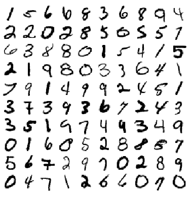
You can read about this dataset by going to the Elements of Statistical Learning website, ESL, then clicking on the “Data” tab, then clicking on the “Info” for the zip code dataset. It is similar to the MNIST dataset (examples shown below):
Use the command less in the terminal to view the beginning of each file:
less /home/smathieson/Public/cs360/zip/zip.train(Use q to exit less.) Both datasets have the same format: the first column is the “label” (here an integer between 0 and 9, inclusive, that corresponds to the identity of a hand-written zip code digit), and the rest of each row is made up of gray-scale values corresponding to the image of this hand-written digit.
One useful technique is to load a dataset from a file into a numpy array. Here is an example:
import numpy as np
train_data = np.loadtxt("path/to/train/file")
In the file lab01.py, test this approach by printing train_data. Make sure the data format makes sense. You can also import the test data in this way. After you load the data, print the shape. The shape of a numpy array represents the dimensions. What is the shape of the training data? Of the testing data?
print(train_data.shape)
print(test_data.shape)
To make this more flexible, we will use command line arguments (similar to many labs in CS260). For this lab -r will represent the training data, -e will represent the testing data, and -d will represent the digit we wish to classify (against all the other digits). For example:
python3 lab01.py -r /home/smathieson/Public/cs360/zip/zip.train -e /home/smathieson/Public/cs360/zip/zip.train -d 5Add a helper function for command line arguments, following this template from CS260 (all arguments should be mandatory):
def parse_args():
    """Parse command line arguments"""
    parser = optparse.OptionParser(description='run linear regression method')

    parser.add_option('-d', '--data_filename', type='string', help='path to' +\
        ' CSV file of data')

    (opts, args) = parser.parse_args()

    mandatories = ['data_filename']
    for m in mandatories:
        if not opts.__dict__[m]:
            print('mandatory option ' + m + ' is missing\n')
            parser.print_help()
            sys.exit()

return optsFor both train and test data, it will be useful to have X (the features) separated from y (the label). Devise a way to accomplish this using numpy array slicing.
To start, we’ll just consider two classes, but here we have 10. We’ll get to such problems later, but for now, devise a way to convert the label to binary based on the user’s input digit. For example, if that value is 5 then:
Using the Logistic Regression documentation, fit a Logistic Regression model to the training data. You may need to increase the number of iterations for gradient descent.
Similarly, using the Naive Bayes documentation, fit a Naive Bayes model to the training data. Think carefully about the features when deciding which type of Naive Bayes model to use.
It is required to have a helpful function that takes in a classifier (along with training data, test data, and optionally other arguments) and runs the model fitting and evaluation process. This is to avoid duplicated code. When thinking about how to design this helpful function (or multiple helper functions), imagine you were training and comparing 10 different classifiers!
For each classifier, predict the labels of the test data. Then compute and print the accuracy, following the rounding format below:
Naive Bayes accuracy: XX.XX%
Logistic Regression accuracy: XX.XX%
You are welcome to use the accuracy score from sklearn.
Following the confusion matrix documentation create and print a confusion matrix for each algorithm. To visualize these results, create a figure for each confusion matrix and save them as following (you may need to create the figs folder):
figs/log_conf_mat.pdf
figs/nb_conf_mat.pdf
See the confusion matrix visualization documentation for more information. The confusion matrix must be normalized to sum to 1 across the rows (true labels), with axis labels and a title. Think about color schemes that follow good visualization principles from CS260.
Finally, create a single plot with two ROC curves comparing Logistic Regression and Naive Bayes. See the CS260 ROC curve lab for a review of this topic.
You are welcome to use the roc_curve function from sklearn here, but the plotting should be done on your own with matplotlib.pyplot. Regardless of how you compute the false positive and true positive rates, you will likely need to use the method predict_proba within each classifier, which returns the prediction probabilities for each class.
Save your plot as shown below. You should have axis labels, a legend, and a title.
figs/roc.pdfMake sure to fill out the README.md with answers to all the analysis questions! (listed below as well) Be sure to commit your work often to prevent lost data. Only your final pushed solution will be graded.
For all 10 digits (0-9), list the accuracies you obtained for Logistic Regression and Naive Bayes.
Based on all your evaluation metrics (accuracy, confusion matrix, ROC curve) which method was better overall? Explain your reasoning.
Credit: based on Chapter 3 of “Hands-On Machine Learning” by Aurélien Géron
If you do any of the extensions, document them in your README.md.
Extend these algorithms and your analysis to a multi-class setting (i.e. distinguish between 3 or more digits). Can we use a ROC curve in this case? A confusion matrix? Push any additional figures and describe your results in your README.md.
Experiment with changing the hyper-parameters of both Logistic Regression and Naive Bayes. How much does this change your results? After informal hyper-parameter optimization, which algorithm performs better?