The goals of this week’s lab:
This week we will be analyzing an Adult Census Income dataset from 1994. The original “label” of this data was the individual’s income (whether less or more than $50k per year). In this lab we’ll be thinking of the data a bit differently.
As we discussed in class, sometimes protected attributes (like race, sex, etc) are redundantly encoded in the data, so ignoring protected attributes is not enough to prevent bias. Here we will see an example of this, and discuss strategies for how to mitigate such effects in the future.
Find your git repo for this lab assignment the lab04 directory. You should have the following files:
run_NB.py - your main program executable for Naive Bayes.NaiveBayes.py - file for the NaiveBayes class.README.md - for analysis questions and lab feedback.Your programs should take in the same command-line arguments as Lab 4 (feel free to reuse this code). For example, to run Naive Bayes on the census example:
python3 run_NB.py -r data/1994_census_cleaned_train.csv -e data/1994_census_cleaned_test.csvTo simplify preprocessing, you may assume the following:
You may assume that all features are discrete (binary or multi-class) and unordered. You do not need to handle continuous features.
Although we are looking at a binary “label” here, make sure your code could handle a multi-class classification task if necessary.
In the starter code you are given an Example class and a Partition class. These are very similar to Lab 4, except that we now have an instance variable for the number of classes K. An instance of an Example holds one row, where the features are represented as a dictionary and the label is represented as an integer. Here is an example (first row of the training data).
age : Senior
workclass : Private
education : HS-grad
marital_status : Widowed
occupation : Exec-managerial
relationship : Not-in-family
race : White
hours_per_week : Part-time
income : <=50K
The “label” we are trying to predict from these features is sex. In this case, the individual is Female, so the label is 1.
A Partition instance holds a list of Examples, as well as the feature dictionary (where each key is a feature name and each value is a list of possible feature values).
To begin, complete the function:
def read_csv(filename):in run_NB.py. This function should return a Partition instance, similar to read_arff from Lab 4. However, in this case we do not have an arff file as input, so we don’t know the possible feature values for each feature. Instead, every time you see a new feature value, add it to the list of values for the appropriate key in F (which will eventually be used to create the Partition instance). A few additional recommendations for this part:
Note that the first row is a header with the feature names. These can be used to initialize the keys of F.
We want to hold aside the feature sex to be used as the label (so you will need a special case for this feature). Here we will use 0 for Male and 1 for Female.
I recommend setting up both F and the feature dictionary for each Example as an OrderedDict(). This will ensure that the keys are always in the same order. To use this functionality you can import:
from collections import OrderedDictcsv package to read in the data. You are also welcome to read in the data another way, for example using numpy arrays or pandas data frames. Here is a way to start your read_csv function (see correction below!)import csv # at the top
csv_file = csv.reader(open(filename, 'r'), delimiter=',')
for row in csv_file:
...To test your read_csv function, you can run the following code:
def main():

    opts = parse_args()
    train_partition = read_csv(opts.train_filename)
    test_partition = read_csv(opts.test_filename)

    # sanity check
    print("num train =", train_partition.n, ", num classes =", train_partition.K)
    print("num test  =", test_partition.n, ", num classes =", test_partition.K)
Here is what the output should be for the census dataset (not the corrected one yet):
num train = 28998 , num classes = 2
num test = 7419 , num classes = 2Now that we have a Partition instance for both the train and test data, we will run some preliminary analyses.
In this lab we will be considering sex as a protected attribute, and seeing if we can predict sex from the remaining attributes. First, compute the fractions of males and females in the training data. Write your numbers in your README.md.
Given these ratios, if an algorithm to predict sex randomly flipped a coin for every test example, what confusion matrix would result? What overall classification accuracy would result? Record in your README.md.
What if an algorithm always predicted the majority class? What would the confusion matrix look like in this scenario? What overall classification accuracy would result? Record in your README.md.
You will implement Naive Bayes as discussed in class. Your model should be capable of making multi-class predictions (i.e. it should work for any K, even though in this case we have K = 2).
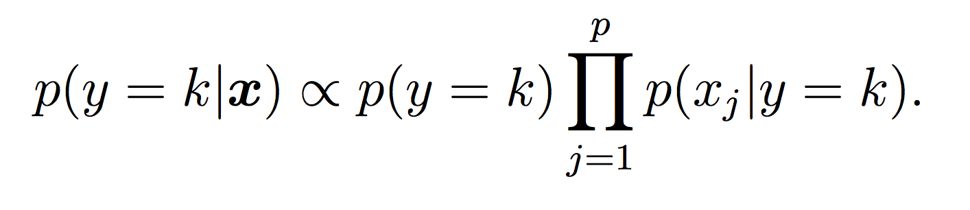
Our Naive Bayes model for the class label k is:
For this lab, all probabilities should be modeled using log probabilities to avoid underflow (depending on your system this might not absolutely be necessary, but it is good practice!) Note that when taking the log of a formula, all multiplications become additions and division become subtractions. First compute the log of the Naive Bayes model to make sure this makes sense.
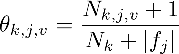
You will need to represent model parameters (θ’s) for each class probability p(y = k) and each class conditional probability p(xj = v|y = k). This will require you to count the frequency of each event in your training data set. Use LaPlace estimates to avoid 0 counts. If you think about the formula carefully, you will note that we can implement our training phase using only integers to keep track of counts (and no division!) Each theta is just a normalized frequency where we count how many examples where xj = v and the label is k and divide by the total number of examples where the label is k (plus the LaPlace estimate):
And similarly for the class probability estimates:
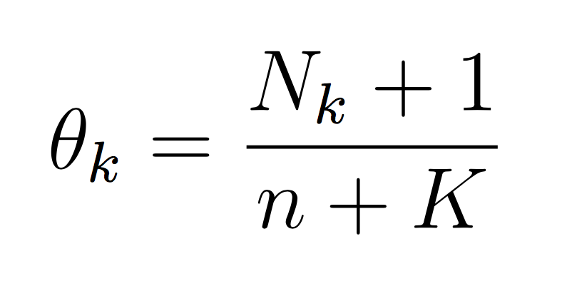
If we take the log then each theta becomes the difference between the two counts. The important point is that it is completely possible to train your Naive Bayes with only integers (the counts, N). You don’t need to calculate log scores until prediction time. This will make debugging (and training) much simpler.
Requirement: the model probabilities should be computed and stored in advance during training, not computed on the fly during testing (which results in duplicated computation).
For this phase, calculate the probability of each class (using the model equations above) and choose the maximum probability:
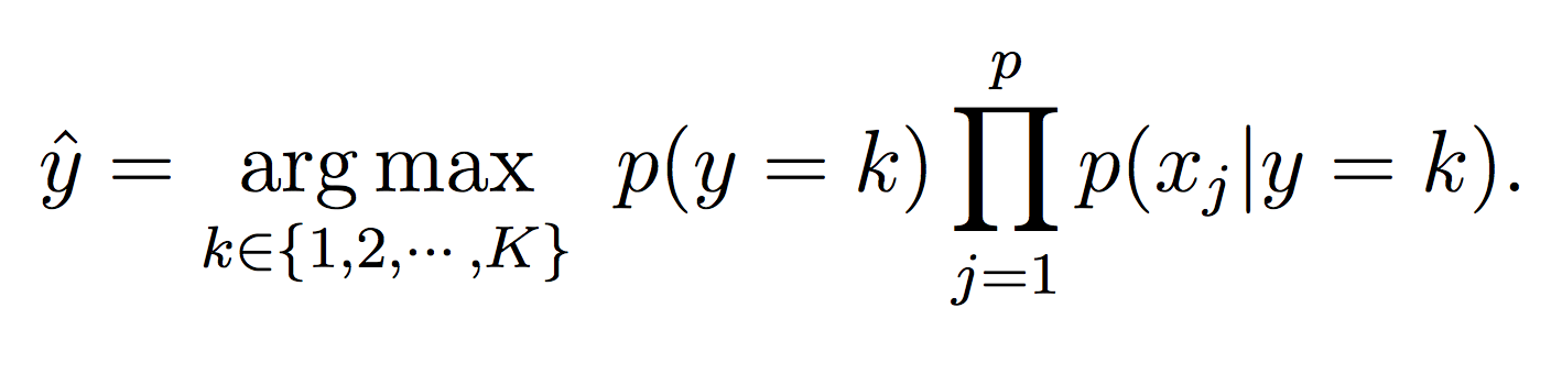
This should be implemented in your classify method.
NaiveBayes class in NaiveBayes.py and do all the work of training (creating probability structures) in the constructor. Then in main, I should be able to do something like:nb_model = NaiveBayes(train_partition)It is okay (and encouraged) to have your constructor call other methods from within the class.
In your NaiveBayes class, you should tally up the number of examples of each class (0 and 1 here, but make it general). This will be used to create the prior probabilities, which should be an instance variable of the class. The type should be a list. To help with debugging, the (log) prior probabilities here should be:
log_prior = [-0.39003307271614496, -1.1302097192251246]For each class and for each feature name, you should also count the number of examples with each feature value from the training data. This will be used to create the likelihood probabilities, which should also be an instance variable. For this type I recommend a dictionary of dictionaries, first indexed by the class and then the feature name.
Both of these data structures should store the probabilities in log space and include LaPlace counts.
classify method within the NaiveBayes class and pass in each test example:y_hat = nb_model.classify(example.features)And compute the accuracy and confusion matrix by comparing these predictions to the ground truth. Here is an example of the format of the output (not for our dataset).
Accuracy: 0.928571 (13 out of 14 correct)

  prediction
     0  1
   ------
 0|  4  1
1| 0 9Answer the following questions in your README.md.
Just temporarily, remove the LaPlace counts from your code and run your method again. What error do you obtain? What does this error actually mean about the data?
When trying to predict sex from the other attributes, what accuracy do you obtain? Is this higher or lower than you would expect with one of the naive strategies from Part 2?
Re-run your method with the corrected train/test data. What accuracy do you obtain now? Explain the difference between the two datasets and why this accuracy change makes sense.
What (if anything) is concerning about being able to predict such a protected attribute from the other attributes (especially using an algorithm like Naive Bayes that does not explicitly account for feature interactions)? If the actual “label” were “hired” or “not hired” for a job, and you were responsible for making this decision, how would you deal with data where features were redundantly encoded?
Devise a way to identify which features (and potentially specific feature values) are most predictive of sex. Write up your strategy and/or results in your README.md.
In these examples, our features were discrete. Devise a way to make Naive Bayes work with continuous features. Discuss your idea in your README.md and/or implement it.
Credit for this lab: modified from materials created by Ameet Soni and Allison Gong.