The goals of this lab:
Credit: Based on materials created by Allison Gong.
In this lab, we will analyze the Mushroom Dataset from the UCI Machine Learning Repository. Each example is a sample of mushroom with 22 characteristics (features) recorded. The goal is to classify the mushroom as “edible” (label -1) or “poisonous” (label +1). In this lab we will use different features to predict edible vs. poisonous and compare the performance using a variety of evaluation metrics. The main deliverable is a ROC curve comparing the performance of the top 5 features.
Note that this lab has some starter code (for reading the data into classes in a particular way), but you are welcome to use your own code instead. This lab is designed to have an intermediate level of structure - there is a roadmap for completing it below, but you are welcome to get to the end goal (ROC curve) in a different way.
To get started, find your git repo for this lab assignment in. You should have the following files:
FeatureModel.py - this is a class representing a model based on a single featurePartition.py - Partition is a class representing a dataset (keeps the features and labels together)run_roc.py - this is the driver for the entire programutil.py - utility program for common functions (you can add to this file)README.md - for analysis questions and lab feedbackThroughout this part make sure you understand how the starter code is working, both in Partition.py and util.py. The files we are using are in arff format, which is different from csv but encodes the same idea. The difference is that the feature names and values are shown at the top. For example, the cap-shape feature name is listed first, along with the possible values:
@attribute 'cap-shape' { b, c, x, f, k, s}These letter abbreviations stand for:
bell=b, conical=c, convex=x, flat=f, knobbed=k, sunken=sThe last “attribute” is the “y” value or label:
@attribute 'class' { e, p}Where e=“edible” (label -1) and p=“poisonous” (label +1).
For run_roc.py, your program should take in the following command line arguments using the optparse library.
train_filename (option -r), the path to the arff file of training datatest_filename (option -e), the path to the arff file of testing dataThis is provided in the starter code (in util.py). So in run_roc.py, call the argument parsing function using util.parse_args(), then read each dataset (train and test) using util.read_arff. This will create two Partition objects. To test this process, you can try:
python3 run_roc.py -r data/mushroom_train.arff -e data/mushroom_test.arffYou can make sure the data is being read in correctly by checking the number of examples in each dataset (use the n member variable):
train examples, n=6538
test examples, m=1586Inside FeatureModel.py we will create a class representing a classification model based on one feature. You should have a main function in this file as well where you test this class. But when you import this file into run_roc.py later on, this main will not be run because we used:
if __name__ == "__main__":
main()In the constructor I would recommend creating a dictionary of probabilities, one for each feature value. Continuing with our cap-shape example, there are 6 possible values - let’s consider the value “bell-shaped” (b). In the training data, 355 examples are bell-shaped. Of these, 41 are poisonous (label +1) and 314 are edible (label -1). So based on the training data alone, we would say that a bell-shaped mushroom has a 41/355 = 11.5% chance of being poisonous.
If we compute these probabilities (i.e. probability of a positive) for all feature values, we would obtain:
{
 'b': 0.11549295774647887,
 'c': 1.0,
 'x': 0.4652588555858311,
 'f': 0.49667318982387476,
 'k': 0.7259036144578314,
 's': 0.0
}
Test this out in your FeatureModel.py file and make sure you can get the same values (you can still use the helper functions in util.py).
Implement the classify method, which classify a single Example and return either +1 or -1, using the given threshold. If the “prob pos” for the feature value (of the Example) is greater than or equal to the threshold, return +1, else return -1.
Now classify all the Examples in the test data and create a confusion matrix. Also compute the accuracy, false positive rate, and true positive rate (all based on the confusion matrix). Make sure to use helper functions or methods.
In your main function inside FeatureModel.py, create the following printout (here you can hard-code the feature “cap-shape” and the threshold=0.5). Don’t worry too much about the formatting of your output, but it should be easily readable by the graders.
$ python3 FeatureModel.py -r data/mushroom_train.arff -e data/mushroom_test.arff

feature: cap-shape, thresh: 0.5

   prediction
      -1    1
   ----------
-1|  785   46
 1|  636  119

accuracy:         0.569987 (904 out of 1586 correct)
false positive:   0.055355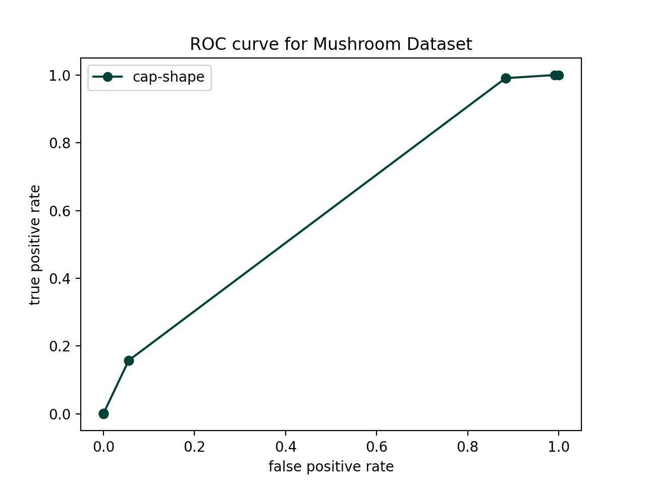
true positive: 0.157616We will now use ROC curves to evaluate the models created from each feature. This will allow us to select the most important (i.e. informative for the label) features. A ROC curve captures both the false positive (FP) rate (which we want to be low), and the true positive (TP) rate (which we want to be high). ROC curves always contain the points (FPR, TPR) = (0,0) and (FPR, TPR) = (1,1), which correspond to classifying everything as negative and everything as positive, respectively. The following steps should help you generate a ROC curve. I would recommend doing most of this in run_roc.py (with use of helpers) but it’s up to you.
cap-shape) and create a model based on this feature. Then choose a variety of thresholds between 0 and 1. I would recommend using the following code (we go slightly below 0 and above 1 to get the terminal points).thresholds = np.linspace(-0.0001,1.1,20)For each threshold, re-classify the test examples and compute the FPR and TPR. This will allow you to build up a list of “x-values” and “y-values” you can plot to create the ROC curve. Test this out for this single feature - you should be able to get a plot like the one below (use "o-" to get the dots connected by lines):
r = random.random()
b = random.random()
g = random.random()
color = (r, g, b)figures folder in your git repo and save your plot as:figures/roc_curve_top5.pdfMake sure to include axis labels, a title, and a legend.
Answer in your README.md.
In this lab we are thinking about poisonous vs. edible mushrooms. For this application, would you prefer a higher or lower classification threshold? Explain your reasoning.
Come up with one example application where you would prefer a low (below 50% threshold) and one where you would prefer a high (above 50% threshold). (Excluding examples from class and from this lab.)
In the main lab we just looked at the ROC curves to determine the best features. Devise a way to compute the area under the curve (AUC) to create a more precise measurement. Which are the top 5 best features now? Write up your AUC method and results in your README.md.
Here we just used one feature at a time. How could you combine these models to create a more robust classification system? Write up you thoughts (and describe any additional code) in your README.md.