Goals:
Credit: Based on materials created by Allison Gong and Jessica Wu.
numpy suggestionsHere are a few suggestions for working through this lab:
If you are seeing many errors at runtime, inspect your matrix operations to make sure that you are adding and multiplying matrices of compatible dimensions. Printing the dimensions of variables with the arr.shape command will help you debug.
When working with numpy arrays, note that numpy interprets the * operator as element-wise multiplication. This is a common source of size incompatibility errors. If you want matrix multiplication, you need to use the np.matmul function. For example, A*B does element-wise multiplication while np.matmul(A,B) does a matrix multiply.
Be careful when handling numpy vectors (rank-1 arrays): the vector shapes (1,n), (n,1), and (n,) are all different things. For simplicity in this lab (unless otherwise indicated in the code), both column and row vectors are rank-1 arrays of shape (n,), not rank-2 arrays of shape (1,n) or (n,1).
Useful numpy functions:
np.array([...]): takes in a list (or list-of-lists, etc) and turns it into a numpy array. Note that after this step, you have to use numpy operations to work with the resulting object.
np.dot(u,v): compute the dot project of two vectors u and v with the same length. Note that this function also works as matrix multiply, but I recommend the following function for clarity.
np.matmul(A,B): multiply the matrices A and B. The inner dimensions must match.
np.ones((p,q)): creates a 2D array of 1’s with the given shape. Similarly, you can use np.zeros((p,q)) to create an array of 0’s. If you include only one dimension (i.e. np.zeros(p)), this will yield a vector.
np.concatenate((A, B), axis=0): concatenate two arrays along the given axis. Here it would be along the rows (axis 0), so A would be “on top”, and B below. In this case A and B do not have to have the same number of rows, but they do have to have the same number of columns. If we concatenate along axis 1 then A would be on the “left” and B would be on the right (and visa versa about the matching dimensions).
np.reshape(A, (p,q)): will reshape array A to have dimensions (p,q) (or whatever dimensions you need, provided the values of A can actually be reshaped in this way).
np.linalg.pinv(A): returns the pseudo-inverse of matrix A (we will use this just in case we have issues with a singular matrix).
Accept your Lab 3 repository on Github classroom. You should have the following folders/files:
linear_regression.py: this is where your code will godata/: folder with three different datasetsTwo of these datasets we have seen before. The USA_Housing dataset is from here and has several features that potentially have an impact on housing prices. In our code we will use the cleaned version of this dataset, but the original is included so you can see the names of the features.
For all these datasets, the features are the first columns and the output (response variable) is the last column.
In this lab we will be using command line arguments. This will allow us to specify the dataset on the command line, as opposed to hard-coding it within the program. As a result, we can change the dataset easily.
Here is example code for command line arguments in Python. Here we have one mandatory argument data_filename.
def parse_args():
    """Parse command line arguments"""
    parser = optparse.OptionParser(description='run linear regression method')

    parser.add_option('-d', '--data_filename', type='string', help='path to' +\
        ' CSV file of data')

    (opts, args) = parser.parse_args()

    mandatories = ['data_filename']
    for m in mandatories:
        if not opts.__dict__[m]:
            print('mandatory option ' + m + ' is missing\n')
            parser.print_help()
            sys.exit()

    return opts
Then in main, we can use this function like this:
opts = parse_args()
filename = opts.data_filename
filename is now a string that we can use later on (i.e. to open the file). On the command line, we can now write:
$ python3 linear_regression.py -d data/sea_ice_data.csvDouble check that this all works correctly on your system, and read the data into a numpy array. Separate X and y into separate variables using numpy array slicing (no loops!)
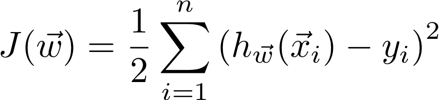
In linear regression, our objective is to minimize the cost function:
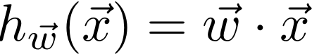
Where our linear model is a dot product of the weights and the features of an example (with a “fake” 1 added to the front of each x).
In class, we learned that the closed-form solution to linear regression is
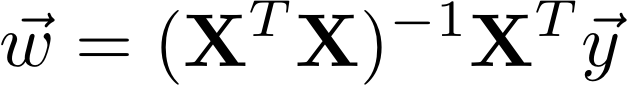
First we will start out by implementing this solution in the function:
def fit(X, y):This should return the optimal weights w (i.e. the model parameters). You may want to add a helper function that adds the column of ones to the X matrix (again using no loops).
Test your analytic method on the sea_ice data and the regression_train data. In your README.md, comment on how close your results are (for w) to the provided models from Lab 2. Make sure your code clearly prints out the weights found by the analytic solution (but no specific format is needed).
NOTE: there should be no for loops in your code! See below for two exceptions in gradient descent.
In this part of the lab we will work with the USA_Housing dataset, as the sea_ice dataset is a bit too small to work well with stochastic gradient descent. Use the steps below as a guide.
First compute the mean and standard deviation for the features (across all examples on the rows, i.e. axis=0).
X_mean = X.mean(axis=0)
X_std = X.std(axis=0)
Then subtract off the mean and divide by the standard deviation to get normalized X values that we will use throughout the rest of the code. Then do the same for the y values.
Implement the functions predict (which should return a vector of predicted y values given a matrix X of features and a vector of weights w) and cost (which should return the value of the cost/loss function J discussed in class). Use your cost function to compute the cost associated with the weights from the analytic solution. This should be roughly the minimum of the cost function J, and will serve as a goal/baseline when implementing gradient descent. (Hint: this value should be around 205.)
Now we will implement stochastic gradient descent in the function:
def fit_SGD(X, y, alpha=0.01, eps=1e-10, tmax=10000):Here alpha is the step size, eps is the tolerance for how much J should change at convergence, and tmax is the maximum number of iterations to run gradient descent. These are the default values, but throughout you’ll need to experiment with these values to ensure efficient convergence. tmax is more of a stop-gap if the method is not converging - it should ideally not be used as a way to stop the algorithm.
During each iteration of SGD, we go through each x_i in turn and update the weights according to the gradient with respect to this x-value.

The goal of this function is to return the final weights after the cost function has converged. To check for convergence, after each iteration of SGD, compute the cost function and compare it to the cost function from the previous iteration. If the difference is less than epsilon (eps), then break out of the loop and return the current weights. You should be able to achieve a cost function value similar to that of the analytic solution.
NOTE: it is okay here to have one for loop over the SGD iterations and one for loop over the examples. Also note that you do not need to randomize the examples for this lab, as would be typical in SGD.
At the end of this step, when run your code should clearly print out:
alpha, eps, and tmax values you used for SGDMake sure in your printout that each value is clearly labeled.
alpha value or debug your algorithm. Save your final plot as:figures/cost_J.pdfIn your README.md, include the optimal weights from both your analytic solution and your SGD solution. Comment on any differences between the two models.
For each model, what was the most important feature? Which features were essentially not important? Do these results make sense to you? Does it matter that we normalized the features first? (include your answers in your README.md)
README.md is completely filled out. Points will be lost for not filling out the last section.In Lab 2 we saw not only linear models, but polynomial models with degrees up to 10. For datasets with a single feature (like sea_ice and regression_train) the machinery of multiple linear regression can actually be used solve polynomial regression.
The idea is to create a matrix X where column k represents x to the power k. Here is what this might look like for a degree d polynomial:
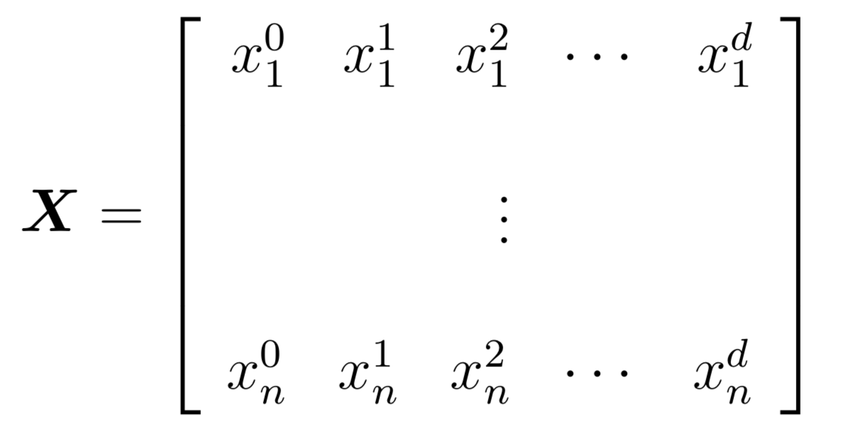
After creating this matrix, we can now run multiple linear regression as usual to find the model, which consists of the coefficients of the polynomial (as opposed to the coefficients of each feature). Try this out and see if you can come up with the polynomial models provided in Lab 2.