Grace period: deadline is flexible
The goals of this week’s lab:
tensorflow and keras)Acknowledgements: adapted from Stanford CS231n course materials
To get started, accept the github repo for this lab assignment. You are encouraged to clone the repo both locally (so you can write the code) and also on the lab machines. That way you can push changes locally, then pull them on the lab machine to run your latest version.
You will have or create the following files:
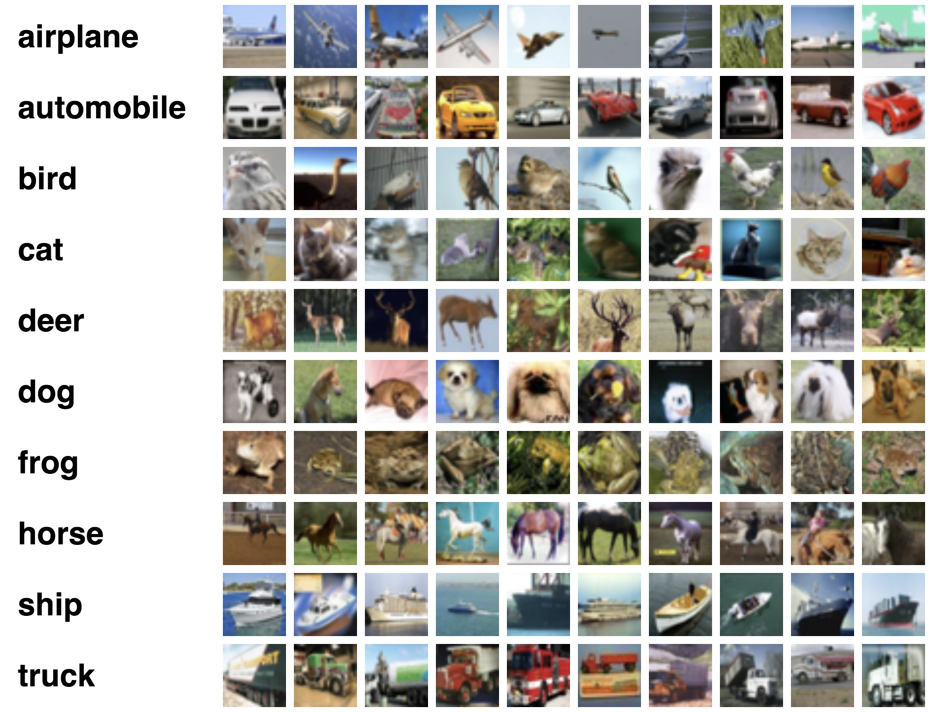
run_nn_tf.py - your main program executable training and testing NNsfc_nn.py - implementation of a fully connected neural networkcnn.py - implementation of a convolutional neural networkrun_best.py - train and test your best neural network (optional)README.md - for analysis questions, results, and data collectionFor this lab, we will be investigating the CIFAR-10 (“see-far”) dataset, which contains small images from 10 classes (examples shown below):
See Learning Multiple Layers of Features from Tiny Images by Alex Krizhevsky (2009) for more information about this dataset.
To use tensorflow, you’ll need to put these lines at the end of your .bashrc file (which should be in your home directory):
export PATH=/packages/cs/python3.7.7/bin:/usr/local/cuda-10.1/bin:$PATH
export LD_LIBRARY_PATH=/usr/local/cuda-10.1/lib64:/usr/local/cuda/extras/CUPTI/lib64:/packages/cs/python3.7.7/lib
We have several machines with GPUs. I will post this list on Piazza (so it is not public), but you do not need to do anything special to use the GPU once you have logged in to one of these machines. If you want to make sure your code is making use of the GPU, you can use:
tf.debugging.set_log_device_placement(True)Similar to Lab 7, we will be using high-level libraries, so consult the documentation frequently. Make sure you really understand each line of code you’re writing and each method you’re using - there are fewer lines of code for this lab, but each line is doing a lot!
When importing modules, avoid importing with the * - this imports everything in the library (and these functions can be confused with user-defined functions). Instead, import functions and classes directly. Imports should be sorted and grouped by type (for example, usually I group imports from python libraries vs. my own libraries).
For help with tensorflow, see the TensorFlow Documentation and Effective TensorFlow 2. Note that your final code will take a while to run, so please budget time for experimenting with different architectures.
1. First, examine the starter code in run_nn_tf.py. There is code for reading in the cifar-10 dataset and dividing it into train data, validation data, or test data. This allows us to iterate over the data in “mini-batches”. In gradient descent, often we use only one data point at a time to update the model parameters. Here we will use mini-batches so that gradient updates are not performed quite so frequently (but also not as infrequently as if we had used the entire “batch”). Mini-batches are a middle ground between these two approaches.
If you are using a laptop instead of the lab computers, download the cifar-10 python data and change the path in run_nn_tf.py to wherever you have downloaded the data.
You don’t need to worry about combine_batches too much - this function reads the data in from a folder and combines data from different files. The load_cifar10 function allows you to choose the number of training, validation, and testing examples. If you are using a laptop instead of the lab computers, reduce the number of training examples so that the program will run on your machine. Here, the input data X has 4 dimensions:
shape of X: (n, 32, 32, 3)where n is the number of examples. Each example is an image of size 32 x 32 pixels. Since we have RGB (red, blue, green) values for each pixel, the depth of the data is 3. We will also refer to 3 as the number of channels.
The first coding step is to modify the load_cifar10 function to subtract off the mean and divide by the standard deviation (normalize the data). This will make our data zero-centered and keep all the features roughly on the same scale (see image below).
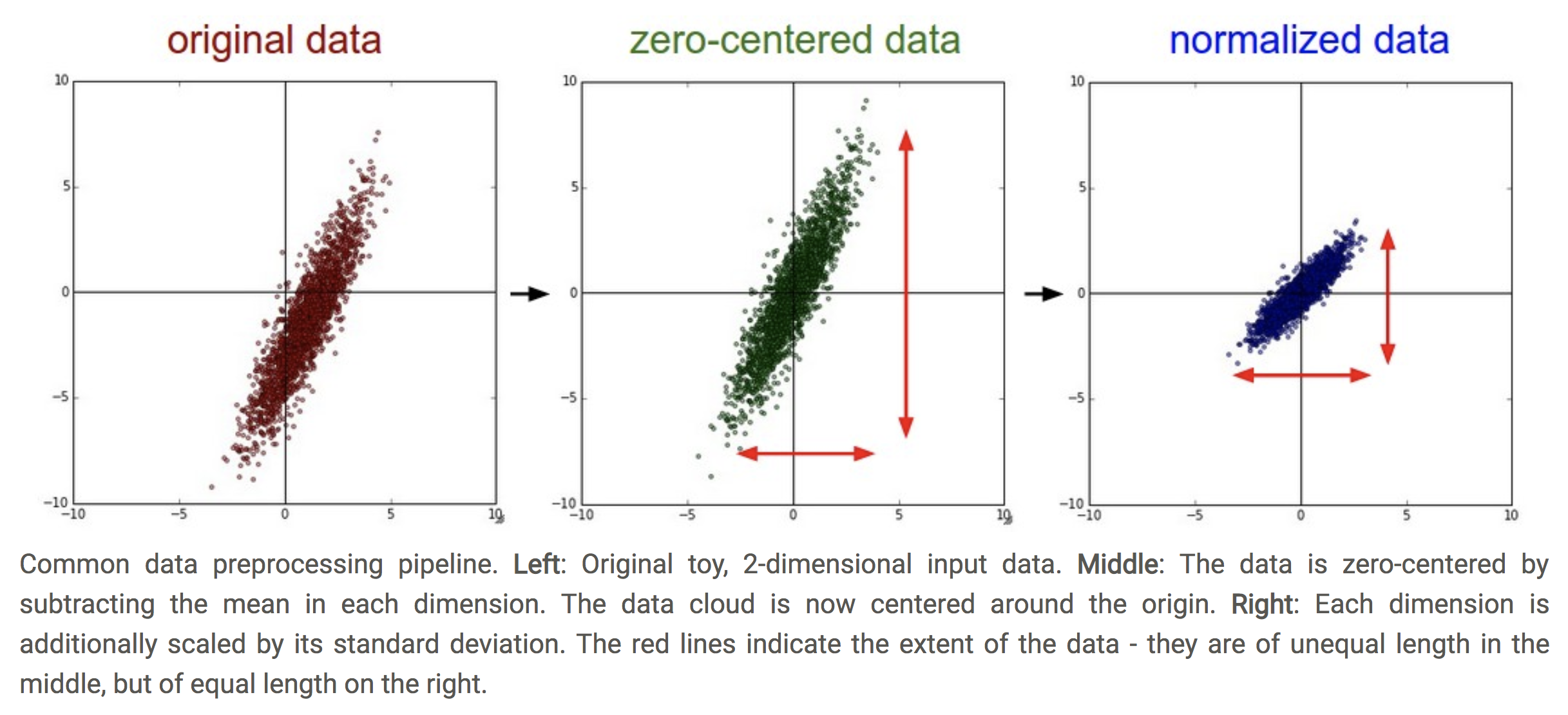
Figure from Stanford CS231n course, section “Neural Networks Part 2: Setting up the Data and the Loss”
We will compute the mean and std on the training data only, since we need to make sure to treat our validation and test data the same way we treated our training data. To perform these operations on a matrix, you can use:
mean_pixel = dset.mean(axis=(0, 1, 2), keepdims=True)
std_pixel = dset.std(axis=(0, 1, 2), keepdims=True)
Where dset should now be the training data. We will compute the mean across the first 3 axes, but allow the RGB channels to have different means. keepdims=True allows the result to be broadcast into the shape of the original data. So after computing these matrices, subtract off the mean matrix and divide by the standard deviation matrix (do this for validation and test data too).
To test this part, run
python3 run_nn_tf.pyAnd make sure you get the dimensions for train, validation, and test as commented in the starter code.
train_dset, val_dset, and test_dset using the tf.data.Dataset.from_tensor_slices method. Here we will use a mini-batch size of 64. We will shuffle the train data, but not the validation and test data. To test this part in main, loop over the train data:for images, labels in train_dset:and print out the shape of images and labels. Do these values make sense?
We are now ready to begin using the data to train neural networks.
fc_nn.py we will implement a fully connected neural network with two layers:Layer one: connect the input nodes to hidden nodes Layer two: connect hidden nodes to the output
Ultimately we will create an FCmodel object. Investigate the documentation for the following types of layers:
tensorflow.keras.layers.Flatten
tensorflow.keras.layers.Dense
In the constructor, we first want to use Flatten to “unravel” an image into a vector of pixels. We want to do this for all images at once, but we don’t want to unravel them all together. So if we have 100 images, each of shape (32,32,3), we want to return a tensor of shape (100,32 * 32 * 3).
Then add two fully connected layers (dense). The first one should have 4000 hidden units and use ReLU activation. The second one should have the number of units matching the number of classes, and use softmax (multi-class logistic regression) as the activation function.
call method that will take an input x (what is the shape of x?), apply the function, and produce the outputs. Each member variable from the constructor is actually a function, so we can apply them to x one at a time until we get to the output (then return this output).To test this part, comment out one of the types of input x_np and run fc_nn.py. What output is produced? Does this output make sense? Switch to the other type of x_np - what does the output look like now?
python3 fc_nn.pyrun_training function in run_nn_tf.py. We can use this function to train any type of model using gradient descent. Work through the TODOs in the starter code to complete this function and the associated helper functions.(Hint: look up documentation for tf.keras.losses and tf.keras.optimizers.)
After each epoch we will check the accuracy on the validation dataset. We will not actually perform hyper-parameter turning here (although you are welcome to do that later), but the idea is that we will not use the testing data until the very end. We use this small validation set to check convergence.
main in run_nn_tf.py, call run_training and pass in the appropriate model and parameters for a 2-layer fully connected network. Then run the code:python3 run_nn_tf.pyTo train the fully connected network on the training data. After a few epochs (pass through all the training data), you should be able to get train accuracies close to 40%. We will return to the fully connected network later for comparison, but for now we turn to a different architecture.
Note: this part is worth less than 15% of the credit - Part 2 is more important.
cnn.py, we will set up the CNN architecture in the class CNNmodel. Our architecture will have two convolutional layers and one fully connected layer. Here is a summary:See the documentation for:
tensorflow.keras.layers.Conv2DRun the function three_layer_convnet_test to confirm the dimensions of your model. Do the results make sense?
python3 cnn.pyrun_nn_tf.py, train a 3-layer neural network using the run_training function with the appropriate input functions and parameters. You can use the same learning rate. After a few epochs you should be able to get over 50% accuracy.One common way to see how training is progressing is to plot accuracy against the training iteration (usually measured in terms of number of epochs). Increase the number of epochs to 10, and then create a plot of both training accuracy and validation accuracy as a function of the training iteration, for both the fully connected NN and the CNN. Here is how the axes should be set up (note you should actually have 4 curves though)!
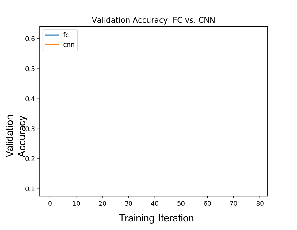
Include this image in your submission (specify which file in your README), along with some brief analysis. Which method did better overall? Do you consider the networks to have converged after 10 epochs? If yes, at what point did they converge?
Note: you can instead make two plots, one for FC and one for CNN (each with two curves, one for train and one for validation).
Devise a way to use your results to create a confusion matrix for the test data (which we so far have not used at all). Include these as either tables or images in your README (one matrix for each method). If you want to copy your results onto a visualization, you are welcome to download the figure below:
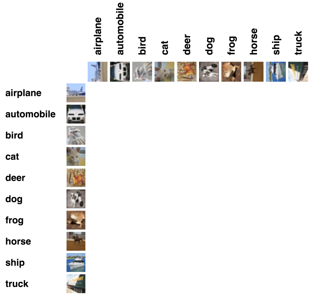
Include brief analysis about which classes seemed the most difficult.
In run_best.py, modify either your fully connected network or your CNN to increase the accuracy on the validation data as much as possible. Suggestions to try:
By the end of this part, you should have improved over the networks in the previous sections. Report your testing accuracy and testing confusion matrix in your README. You should be able to get at least 60-65% accuracy on the test data. Briefly discuss what you tried and what had the biggest impact in your README. Make sure to use the machines with GPUs for faster training!
One more optional idea: set up a runtime comparison between GPU machines and your laptop (or another machine with a CPU). On the command line put the keyword time in front of your command to get the overall runtime.