The goals of this lab:
Note that this lab has a checkpoint: by lab on Thursday Oct 31 you should have completed at least Part 1 and Part 2, and be able to demonstrate this functionality to me during lab.
In this lab, we will analyze the Mushroom Dataset from the UCI Machine Learning Repository. Each example is a sample of mushroom with 22 characteristics recorded. The goal is to classify the mushroom as “edible” (label -1) or “poisonous” (label +1). In this lab we will compare the performance of Random Forests and AdaBoost on this dataset. The main deliverable is a ROC curve comparing the performance of these two algorithms.
Note that this lab has some starter code (for creating Decision Stumps and reading arff files in a particular way), but you are welcome to use your own code instead. This lab is designed to have an intermediate level of structure - there is a roadmap for completing it below, but you are welcome to get to the end goal (ROC curve) in a different way.
To get started, find your git repo for this lab assignment in:
$ cd cs360/lab06/You should have the following files:
random_forest.py - your main program executable for your Random Forest algorithm.ada_boost.py - your main program executable for your AdaBoost algorithm.util.py - utility program for common methods (you should add to this file).roc_curve.py - program for running Random Forest and AdaBoost to create a ROC curve.DecisionStump.py - algorithm for creating Decision Stumps (complete and add a main).Partition.py - class to hold a partition of data (you will add weighted entropy).README.md - for analysis questions and lab feedback.For random_forest.py and ada_boost.py, your program should take in command line arguments using the optparse library. For random_forest.py and ada_boost.py, we will have 4 command line arguments:
train_filename (option -r), the path to the arff file of training datatest_filename (option -e), the path to the arff file of testing dataT (option -T), the number of classifiers to use in our ensemble (default = 10)thresh (option -p), the probability threshold required to classify a test example as positive (default = 0.5)I would recommend putting argument parsing in your util.py file. To test (i.e. in random_forest.py), you can try:
python3 random_forest.py -r data/mushroom_train.arff -e data/mushroom_test.arff -T 20 -p 0.2Right now -T and -p don’t do anything, but you can make sure the data is being read in correctly by checking the number of examples in each dataset (use the n member variable):
train examples, n=6538
test  examples, m=1586
For the command line arguments, make sure to include a program description (you can even pass this in to parse_args(..)), provide help messages for the arguments, and then have opts be the return value from parse_args(..).
To become more familiar with the DecisionStump.py code, complete the classify method. This should return 1 if the probability of a positive label is greater than or equal to the provided threshold, and it should return -1 otherwise. (Hint: doesn’t need to be recursive.)
Next, implement weighted entropy in the Partition class (inside Partition.py). (Note that you can move on to Random Forests if you like, since they do not require weighted entropy, but I recommend doing this part first since it will help you become more familiar with the starter code.)
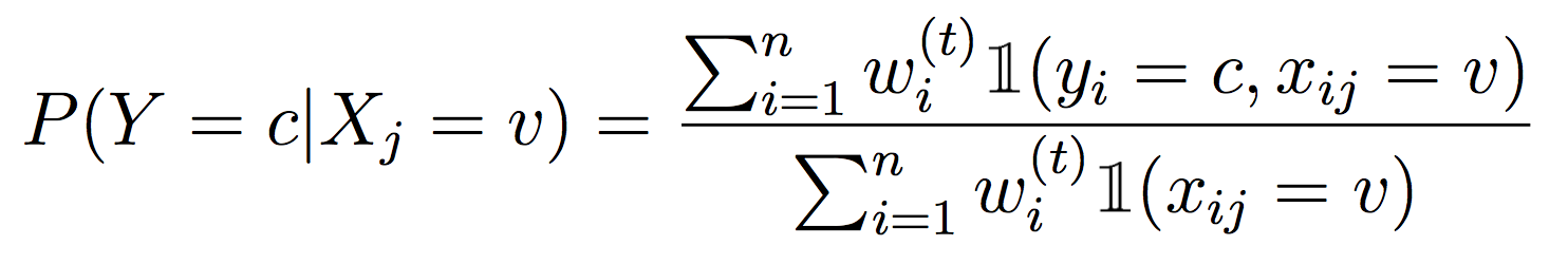
Recall from class that to properly weight examples with Decision Trees, we need to compute weighted entropy and information gain. I recommend copying over your probability and entropy methods from Lab 2, then modifying them to work with the Partition data structure and weighted examples. For each method that computes a probability, we need to weight the counts, i.e.
And for the leaves, we will weight the examples that fall into each feature value:
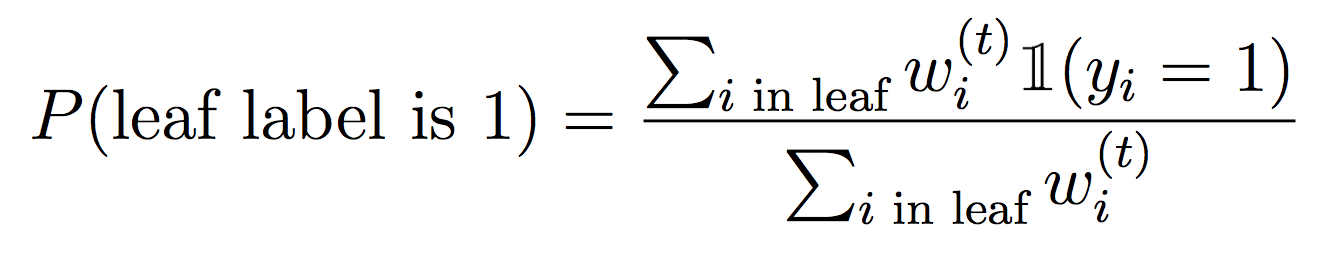
Concretely, to make the DecisionStump data structure work, you’ll need to implement best_feature(..) (using weighted info gain) as well as prob_pos(..) to compute the probability of assigning a positive label at a leaf.
To check that your method is working, I recommend using the tennis dataset (note the train and test are the same, not very realistic!) Inside your DecisionStump.py file, create a main that is only executed when we run the program from the command line. Then read in the tennis train and test data and create a decision stump. With no re-weighting of the examples, you should be able to generate this output:
$ python3 DecisionStump.py
TRAINING
Info Gain:
     Outlook, 0.246750
 Temperature, 0.029223
    Humidity, 0.151836
        Wind, 0.048127

D-STUMP
Outlook =
  Sunny, 0.4
  Overcast, 1.0
  Rain, 0.6000000000000001

TESTING
 i   true  pred
 0  -1  -1
 1  -1  -1
 2   1   1
 3   1   1
 4   1   1
 5  -1   1
 6   1   1
 7  -1  -1
 8   1  -1
 9   1   1
10   1  -1
11   1   1
12   1   1
13  -1   1
error = 0.2857
(You do not need to format your output, this is just for testing).
To break this down, the first part computes the info gain for each of four features. Since “Outlook” produces the maximum info gain, we choose it as the one feature for our decision stump.
The resulting decision stump classifier is shown next, using the print(..) function since we have a __str__ method. The numbers next to each feature value are the probability of classifying a new dataset as positive. So if we had a test example with “Outlook=Sunny”, we would probably classify it as negative (i.e. we don’t play tennis), but if we had a lower threshold (i.e. 0.25), we might still decide to play.
The next part is the classification of each test example, based on this decision stump (for a threshold of 0.5).
Now, to make sure weighted entropy is working, you can use the following code to re-weight the training data (right after you read it in):
for i in range(train_partition.n):
    example = train_partition.data[i]
    if i == 0 or i == 8:
        example.set_weight(0.25)
    else:
        example.set_weight(0.5/(train_partition.n-2))
Then if you run your testing code again, you should get a different decision stump with feature “Humidity”:
$ python3 DecisionStump.py
TRAINING
Info Gain:
     Outlook, 0.154593
 Temperature, 0.274996
    Humidity, 0.367321
        Wind, 0.006810

D-STUMP
Humidity =
  High, 0.24999999999999994
  Normal, 0.9166666666666667

TESTING
 i   true  pred
 0  -1  -1
 1  -1  -1
 2   1  -1
 3   1  -1
 4   1   1
 5  -1   1
 6   1   1
 7  -1  -1
 8   1   1
 9   1   1
10   1   1
11   1  -1
12   1   1
13  -1  -1
error = 0.2857
Throughout this part make sure you understand how the starter code is working, both in DecisionStump.py and util.py.
You will implement the Random Forests as discussed in class, for the task of binary classification with a label in {-1, 1} (you may assume this throughout the lab).
At a high level, random forests create many decision stumps (or any other weak classifiers) by both randomly selecting training examples with replacement (bootstrap) and randomly selecting subsets of features. This help de-correlate classifiers and make them more diverse. For each classifier (T total), repeat the following steps:
Create a bootstrap training dataset by randomly sampling from the original training data with replacement. You are welcome to do this in util.py or random_forest.py. For this lab, we will select n examples (so the bootstrap dataset and the original dataset have the same size).
Select a random subset of features. For this lab, we will select sqrt(p) features (rounded to the nearest integer), where p was the original number of features (in this case 22). For this part, we do NOT sample features with replacement, they should all be unique. If we had kept all the features, this is called bagging.
Using the bootstrap sample and the subset of features, create a decision stump. Add this to your ensemble of decision stumps. We will use this ensemble to vote on the label for each test example.
Repeat these three steps T times. Make sure to separate your training procedure from your testing procedure and use good top-down-design principles!
For each test example, run it through each classifier in your ensemble and record the result (-1 or 1). This testing should be based on the user-supplied threshold (-p). There are several ways to apply the threshold, but for this lab, we will use the threshold with each individual classifier. Then for the final output, we will use a majority vote (so if the number of votes for -1 is equal or greater than the number of votes for 1, we say the classification is negative, else positive).
After that, compute a confusion matrix, as well as the false positive rate and the true positive rate (these would be great functions to put in util.py). Your final output should look something like this (I’ve shown two examples with the same parameters, your numbers will be slightly different).
$ python3 random_forest.py -r data/mushroom_train.arff -e data/mushroom_test.arff -T 20 -p 0.3

T: 20 , thresh: 0.3

   prediction
      -1    1
   ----------
-1|  711  120
 1|   70  685

false positive: 0.1444043321299639
true  positive: 0.9072847682119205
$ python3 random_forest.py -r data/mushroom_train.arff -e data/mushroom_test.arff -T 20 -p 0.3
T: 20 , thresh: 0.3
prediction
-1 1
----------
-1| 647 184
1| 0 755
false positive: 0.2214199759326113
true positive: 1.0Note that this low threshold is conservative and pushes many examples to be labeled as positive (poisonous). So we obtain a high true positive rate, but at the expense of many “false alarms”. The ideal threshold will depend on the application.
You will implement the AdaBoost (adaptive boosting) algorithm as discussed in class. We will again only consider the binary classification task with labels in {-1, 1}.
In ada_boost.py, implement the AdaBoost algorithm. Note that traditionally we will not use bootstrap resampling in AdaBoost, as we want the training data and corresponding weights to be consistent throughout the process. See Handout 9 for more details, but briefly, we will repeat the following steps for each iteration t = 1, 2, …, T:
Train a classifier (decision stump here) on the full weighted training dataset. The result will be a decision stump that we will add to our ensemble.
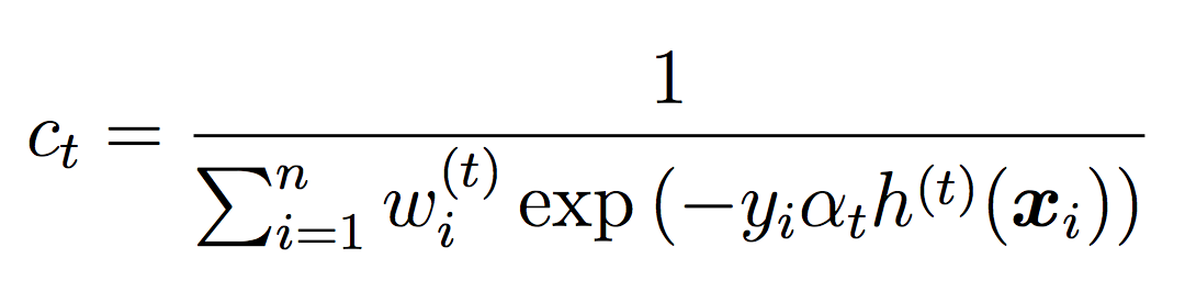
Compute the weighted error of this classifier on the training data:
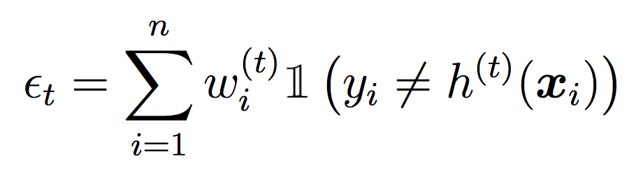
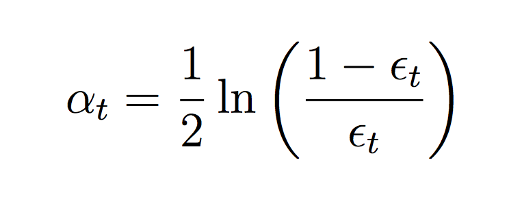
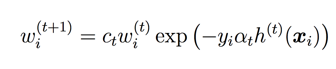
where ct is a normalizing constant that ensures the weights sum to 1.
Note that we will not use the threshold during training (we will use the default of 0.5). The threshold will only be used for testing and evaluation.
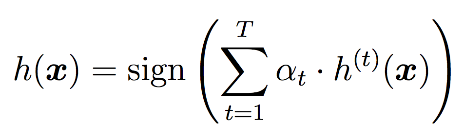
We will again use all the classifiers for testing, but this time we will weight their votes differently depending on how well they did during training. As we did in Random Forests, for testing we will use the threshold for each individual classifier, then take the sign of the final result as our label.
Here is an example output with 20 stumps and a threshold of 0.3. Since our implementation of AdaBoost does not involve randomness, you should be able to reproduce these results.
$ python3 ada_boost.py -r data/mushroom_train.arff -e data/mushroom_test.arff -T 20 -p 0.3

T: 20 , thresh: 0.3

   prediction
      -1    1
   ----------
-1|  290  541
 1|    0  755

false positive: 0.6510228640192539
true positive: 1.0To compare these two algorithms, this time we will use ROC curves. A ROC curve captures both the false positive (FP) rate (which we want to be low), and the true positive (TP) rate (which we want to be high). ROC curves always contain the points (FP, TP) = (0,0) and (FP, TP) = (1,1), which correspond to classifying everything as negative and everything as positive, respectively. The following steps should help you generate a ROC curve.
roc_curve.py, import both random_forest and ada_boost, as well as util. You can hard-code the dataset, but you should allow the user to choose one parameter, the number of trees. So I should be able to run your code with:python3 roc_curve.py -T 3to generate a plot with ROC curves for both Random Forest and AdaBoost.
Run your training procedures for both Random Forest and AdaBoost, generating ensembles of classifiers (does not rely on a threshold). Note that AdaBoost changes the weights on examples, so you either need to run Random Forest first, or reset the example weights after AdaBoost.
For a list of thresholds in [0,1], run testing using the two ensembles. Training is fairly quick so you can be liberal about how many thresholds you use - this will help generate a smooth ROC curve. I would suggest at least 10 thresholds. One note - you may need to also use a threshold slightly higher than 1 and/or slightly less than 0 to ensure you get the terminal points of the ROC curve (due to the way we break ties in classification). But your FP and TP rates should always be in [0,1].
Save the FPs as the x-values and the TPs as the y-values, then create a plot with the same structure as the one below (note that these are not ROC curves in any sense! they just give an idea of the plot structure). See Lab 2 for an example of code to generate such a plot.
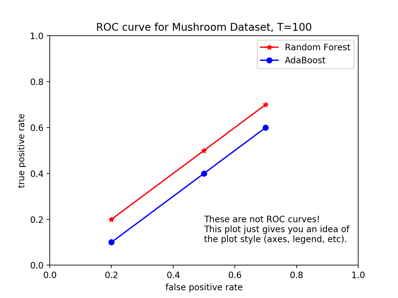
figs folder in your git repo and save your plots as:figs/rf_vs_ada_T10.png
figs/rf_vs_ada_T100.pngBased on your ROC curves, which method would you choose for this application? Which threshold would you choose? Does your answer depend on how much training time you have available?
T can be thought of as a measure of model complexity. Do these methods seem to suffer from overfitting as the model complexity increases? What is the intuition behind your answer?
Perform an analysis of how the performance of each method changes as T is varied. My suggestion for this is to use AUC (Area Under the [ROC] Curve).
Devise a way to evaluate performance as the amount of training data is varied (this could include modifying the number of bootstrap examples).
Incorporate cross-validation into your algorithm to choose the hyper-parameters T and the classification threshold.