CS364 Lab 6: Perfect Phylogeny and Parsimony

Overview and goals

By the end of this lab you should be able to:

Understand and implement Gusfield’s Perfect Phylogeny algorithm
Understand and implement Sankoff’s Weighted Parsimony algorithm
Demonstrate the correctness of the theoretical runtimes of Gusfield’s algorithm

Part 1: implement Gusfield’s algorithm

Clone your Lab 6 git repo as usual. You should see following starter files:

README.md - questionnaire to be completed for your final submission
gusfield.py - where you should implement Gusfield’s algorithm
sankoff.py - where you should implement Sankoff’s algorithm
runtime.py - where you should devise a way to compare the runtime of Gusfield’s algorithm and a naive algorithm
data/ directory - input files

You are welcome to add additional python files as long as the top-level files are the same.

Usage and input data

Perfect phylogeny should take in 2 command-line arguments using the optparse library. You are welcome to add a small number of additional arguments, but make sure they are clearly documented (i.e. when I run your program with no arguments a helpful message is produced). For example, you might want to add a command-line argument for the number of sites (or samples) to analyze.

The name of the file containing the binary matrix M -m
The name of the output file where the tree image should be written -t

The input file has the samples as rows and the sites as columns (see in-class example below). This is actually not typical of genomic data file formats, since there are typically many more sites than samples. But to be consistent with what we’ve done in class we’ll write the matrices this way:

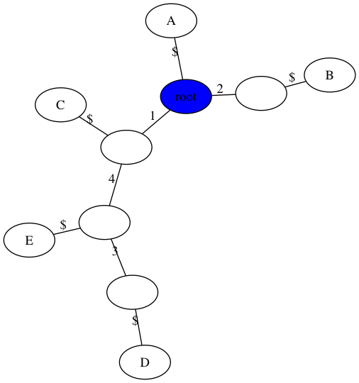
Handout 15, Example 2:

You may assume the data is in the right format and only contains 0’s and 1’s.

Examples

The output below is minimal and should be used a guideline. You are welcome to include intermediate output, but make sure it’s not overwhelming (test on the larger examples at the end). You should output a tree in pygraphviz format (or another format like networkx is fine).

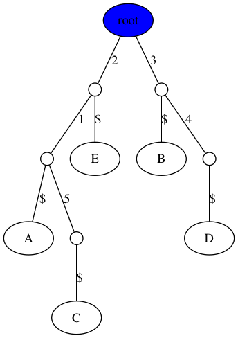
Handout 15: Example 1

$ python3 gusfield.py -m data/inclass1.matrix -t figs/inclass1.png
----------------------------
Welcome to Perfect Phylogeny
----------------------------

number of samples, n = 5
number of sites, m = 5

Perfect Phylogney? True
number of repeated mutations: 0

Handout 15: Example 2

$ python3 gusfield.py -m data/inclass2.matrix -t figs/inclass2.png
----------------------------
Welcome to Perfect Phylogeny
----------------------------

number of samples, n = 5
number of sites, m = 4

Perfect Phylogney? True
number of repeated mutations: 0

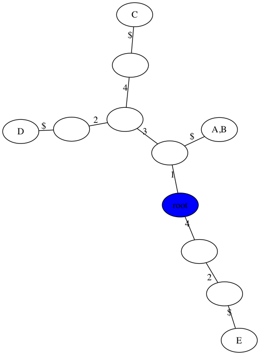
Extra example without a perfect phylogeny

$ python3 gusfield.py -m data/extra.matrix -t figs/extra.png
----------------------------
Welcome to Perfect Phylogeny
----------------------------

number of samples, n = 5
number of sites, m = 4

Perfect Phylogney? False
number of repeated mutations: 2

Implementation requirements and suggestions

There are three main steps to implementing Gusfield’s algorithm:

Radix sort the columns of the matrix. ~~Although we have binary data here, your implementation of radix sort should be general for any alphabet.~~ Edit: you can assume the alphabet is {0,1}. You should implement radix sort from scratch without using any built-in sorting functions.
Rewrite the rows of the matrix as the list of columns containing a 1.
Create a keyword tree (also called trie) from the rewritten rows. Hint: what type of function would be more natural for this step? In the process of creating this keyword tree, you should also create a visualization which can be written to a file.

After implementing these steps, devise a way to determine if there is a perfect phylogeny or not. You should print this result, along with the number of repeated mutations. I would recommend using a class for your perfect phylogeny algorithm, but it is not required.

Note: your trees do not have to look exactly like this. You are welcome to omit the $ character in the visualization or make the root at the “top” (see extra credit from last week). You can also change the size of internal nodes or collapse non-branching nodes into a single edge. Also, I used 0-based indexing for the sites in implementation, and just added one to the edge labels to make the tree consistent with our in-class work.

Output and analysis

You should run your implementation on the three examples above, as well as the file here:

/homes/smathieson/Public/cs364/sim_n100.matrix (m=1359729)

This is a large file so I would recommend running your algorithm on a subset of the sites (i.e. the first x sites). This dataset is simulated with over 1 million polymorphisms. For now just make sure you can run your algorithm on a subset of the sites. This dataset is mainly for use in the runtime analysis section below.

In terms of what to submit, you do not need to create and push a figure for the simulated data.

Part 2: implement Sankoff’s Algorithm

For the second part of your lab, we will perform ancestral state reconstruction using parimony. In a file called sankoff.py, write a program with the following objective:

Given:

a tree (i.e., file of edges between nodes)
sequences for each leaf in the tree
cost matrix for substitutions

Do:

score the tree for its minimum cost using weighted parsimony (i.e., Sankoff’s algorithm)
infer the most likely sequence for each ancestor in the tree
output the score and resulting inferred phylogeny

An example run of your program:

python3 sankoff.py -t tree -s substitution_matrix -l leaf_sequences

Input File Formats

Leaf Sequences: Contains a list of all of the n sequences representing the leaves of the tree. Each line will be in the format:

id: sequence

where id is the name of the organism or gene, and should match a leaf in the tree input file (below). sequence is a DNA sequence. The file data/wp_inclass.seq is the in-class example we did, with the leaves labeled as L1 through L4.

Tree File: The tree file will define the topology of the phylogenetic tree you are attempting to score. The first line specifies the root. Each line after that is in the format:

child parent

For example, the tree from class (data/wp_inclass.tree) would be:

N1
N2 N1
N3 N1
L1 N2
L2 N2
L3 N3
L4 N3

N1 is the root, and has two children N2, N3.

Weighted Cost Matrix: Specifies the substitution value for each pair of states possible at each position in the sequence. This has the exact same format as the distance matrix in the neighbor joining algorithm; that is, each line contains a pair of characters followed by their substitution score. You can find the example from class in data/wp_inclass.cost. The diagonal is not defined, but you should set it to 0 when you create your cost function.

Output

Your program should print the total tree score as well as the inferred state of all common ancestors after running the weighted parimony algorithm. Each line should be specified as:

id: sequence

similar to the input sequence file. Here is an example run with the in-lecture example:

python3 sankoff.py -t wp_inclass.tree -s wp_inclass.cost -l wp_inclass.seq

Score: 9.0

Inferred States:
L4: G
L2: C
L3: T
L1: A
N1: T
N2: T
N3: T

For debugging purposes, you should output intermediate calculations. You can see my intermediate outputs here. When submitting, please remove this intermediate prints or ensure the required output appears at the end of the file.

Tip: Representing Trees

While you can construct a tree data structure to help implement your program, it is probably easier to use a dictionary instead. For example you can have a dictionary where the key is the node identifier (e.g., "N1") and the value is a list of the children (e.g., ["N2","N3"]). A leaf node simply has an empty list for its value. If you need to represent parents, you can have a companion dictionary where the keys and values are reversed.

Multi-Character Sequences

You should first get your program to work on single-character sequences as practiced in class. Once that is complete, you will want to improve your algorithm to calculate the cumulative score and trace for a set of sequences of length m. You can assume that each leaf sequence is of the same length. Also, since we assume independence of positions, you should be able to just place a loop around the function you already created (you are practicing modularity, right?). I have given a second set of example files beginning with the prefix mammals. A sample run will output:

python3 sankoff.py -t mammals.tree -s mammals.cost -l mammals.seq
Score: 11.0

Inferred States:
Aardvark: CAGGTA
Chimp: CGGGTA
Dog: TGCACT
Bison: CAGACA
Elephant: TGCGTA
C3: CGGGTA
C2: TGCGTA
C1: CAGGTA
C4: CGCGTA

An output of intermediate values can be found here.

Part 3: Runtime Analysis

One way of determining if there is a perfect phylogeny is to look at all pairs of columns i, j and see if O_i and O_j are disjoint or one contains the other. In the runtime.py file, implement this approach, which we will refer to as the “naive algorithm” although it makes use of a non-trivial observation about perfect phylogenies. Then compare the runtime of the naive algorithm to Gusfield’s algorithm, in terms of the number of sites.

Requirements

Use the /homes/smathieson/Public/cs364/sim_n100.matrix dataset, which represents a “worst-case” runtime scenario for the naive algorithm.
Exclude the tree drawing part from the runtime analysis - the goal is just to get to a yes/no answer about the perfect phylogeny.
You can use the time module as we did before. Your final output should be a matplotlib graph with the number of sites m on the x-axis and the runtime of each algorithm on the y-axis. Make sure to include axis labels, a legend, and a title.
Finally, answer the questions in the README about the runtime analysis (namely, does your plot agree with the theory?)

Additional requirements

Your program should follow good design practices - effective top-down design, modularity, function/method headers, file headers, and comments.
Use variable names that mirror our in-class notation as closely as possible. This is not only to make your code easier to write, but easier for someone else to read.
You may submit as many additional files as you wish.
Do not interact with the user for your program.
Clean up any debugging print statements.

Analysis and Submitting your work

Make sure to push your code often, only the final version will be submitted. The README.md file asks a few questions about the runtime analysis. Answer these questions and make sure to push the following files. I would recommend making a figs directory for the figures. It is very helpful if you name your figures the same as below - thanks!

README.md
gusfield.py
sankoff.py
runtime.py
figs/inclass1.png, figs/inclass2.png, figs/extra.png
figs/runtime.png (runtime figure)

Credit for weighted parsimony section: Ameet Soni