In this lab you will implement your own de Bruijn graph assembler and apply it to a realistic (although synthetic) dataset. The goals of this lab are to develop a deeper understanding of de Bruijn graphs, gain experience going from theory to application, and understand the limitations of our current assembly tools.
Your program should be broken into two files. The first, debruijn.py will contain class definitions for your de Bruijn graph data structure. The second, assembly.py will be your main program that will orchestrate building, traversing, and interpreting the de Bruijn graph.
In your GitHub repo you should see the starter program files, as well as some example datasets. The first step is to construct a de Bruijn graph for a set of reads (in the FASTA file format). After creating the de Bruijn graph, we will traverse it to create contigs, which can then be written to a file. Some examples of the program execution are shown below to help you get an idea of what your program should do. They are explained in more detail below.
Here is some output from test1.fasta with k=3:
$ python3 assembly.py -r data/test1.fasta -k 3 -o results/test1
----------------------------------------
Welcome to the de Bruijn graph assembler
----------------------------------------
Creating de Bruijn graph with k=3...
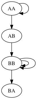
Nodes: AA,AB,BA,BB
Edges:
AA: ['AA', 'AB']
AB: ['BB']
BB: ['BB', 'BB', 'BA']
Graph Eulerian? True
Starting path 1 / 1 from AA:
AAABBBBAThere should be two output files: results/test1_contigs.fasta and results/test1.png with a visualization of the graph. It should look like this:
Here is some output from test2.fasta with k=5:
$ python3 assembly.py -r data/test2.fasta -k 5 -o results/test2
----------------------------------------
Welcome to the de Bruijn graph assembler
----------------------------------------
Creating de Bruijn graph with k=5...
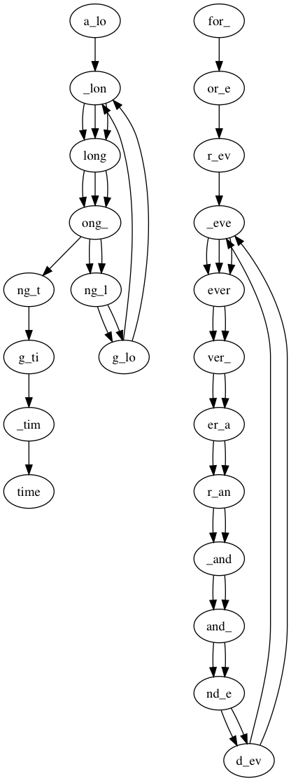
Nodes: _tim,g_ti,for_,er_a,ng_t,r_ev,long,nd_e,time,r_an,_lon,g_lo,a_lo,ver_,d_ev,ever,_eve,ng_l,_and,ong_,and_,or_e
Edges:
a_lo: ['_lon']
_lon: ['long', 'long', 'long']
long: ['ong_', 'ong_', 'ong_']
ong_: ['ng_l', 'ng_l', 'ng_t']
ng_l: ['g_lo', 'g_lo']
g_lo: ['_lon', '_lon']
ng_t: ['g_ti']
g_ti: ['_tim']
_tim: ['time']
for_: ['or_e']
or_e: ['r_ev']
r_ev: ['_eve']
_eve: ['ever', 'ever', 'ever']
ever: ['ver_', 'ver_']
ver_: ['er_a', 'er_a']
er_a: ['r_an', 'r_an']
r_an: ['_and', '_and']
_and: ['and_', 'and_']
and_: ['nd_e', 'nd_e']
nd_e: ['d_ev', 'd_ev']
d_ev: ['_eve', '_eve']
Graph Eulerian? False
Starting path 1 / 2 from for_:
for_ever_and_ever_and_ever
Starting path 2 / 2 from a_lo:
a_long_long_long_timeThere should be two output files: results/test2_contigs.fasta and results/test2.png with a visualization of the graph. It should look like this:
Here is some output from test3.fasta with k=3:
$ python3 assembly.py -r data/test3.fasta -k 3 -o results/test3
----------------------------------------
Welcome to the de Bruijn graph assembler
----------------------------------------
Creating de Bruijn graph with k=3...
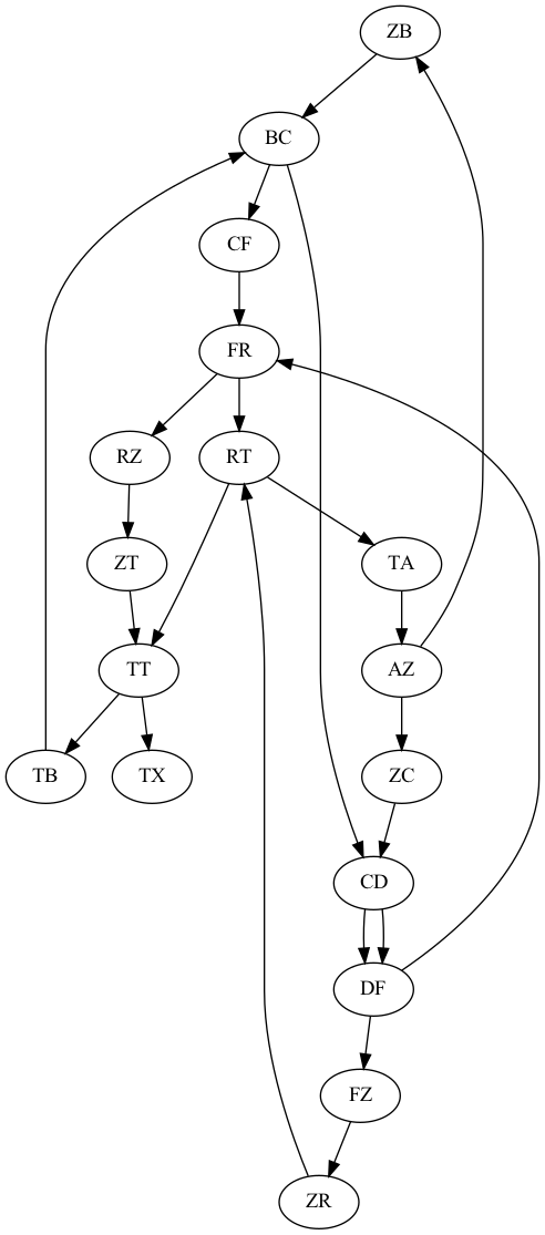
Nodes: TA,AZ,BC,ZT,TB,ZB,CD,CF,ZC,RZ,DF,TT,TX,RT,FR,ZR,FZ
Edges:
AZ: ['ZB', 'ZC']
ZB: ['BC']
BC: ['CD', 'CF']
CD: ['DF', 'DF']
DF: ['FZ', 'FR']
FZ: ['ZR']
ZR: ['RT']
RT: ['TT', 'TA']
TT: ['TB', 'TX']
TB: ['BC']
CF: ['FR']
FR: ['RT', 'RZ']
TA: ['AZ']
ZC: ['CD']
RZ: ['ZT']
ZT: ['TT']
Graph Eulerian? True
Starting path 1 / 1 from AZ:
AZCDFRZTTBCFRTAZBCDFZRTTXThere should be two output files: results/test3_contigs.fasta and results/test3.png with a visualization of the graph. It should look like this:
For this program we’ll start using the optparse library library for parsing command line arguments. Below is some boiler-plate code I use for almost every script I write in Python. It allows you to specify command line arguments with flags so the order of arguments does not matter.
import optparse
import sys

parser = optparse.OptionParser(description='program description')

parser.add_option('-a', '--arg1', type='string', help='helpful message 1')
parser.add_option('-b', '--arg2', type='int',    help='helpful message 2')

(opts, args) = parser.parse_args()

# you can include any subset of arguments as mandatory
# (if an argument is not mandatory, it should have a default)
mandatories = ['arg1', 'arg2']
for m in mandatories:
    if not opts.__dict__[m]:
        print('mandatory option ' + m + ' is missing\n')
        parser.print_help()
        sys.exit()

# later on in your code...
print(opts.arg1, opts.arg2)
For this lab you should have three command line arguments:
-r: the input file of reads in fasta format (string)-k: the k-mer length (int)-o: the prefix for output files (we will add .png for the visual and _contigs.fasta for the output sequences). This is also a string.In the file debruijn.py you will define your de Bruijn graph data structure. At minimum, you should have a class for the de Bruijn graph (i.e. DBG). The methods below provide some guidance, but as long as you’re implementing a de Bruijn graph you’re welcome to make some reasonable modifications.
Note: you must have some testing in the main function in debruijn.py. I would recommend hard-coding test1.fasta for this part. Use if __name__ == "__main__": to prevent this testing from being executed when you import these classes into assembly.py. Make use of assert to ensure you’re getting the results you expect in your tests.
Create a DBG class with the following functionality. Note that the reads should be read in from a FASTA file. All the reads in the FASTA file will be part of the same de Bruijn graph, which will (hopefully) be connected across reads.
A constructor that creates the nodes and edges of the graph. I would recommend two parameters for the constructor: the FASTA filename (i.e. test1.fasta) and the k-mer length.
Instance variables for nodes and edges. This is up to you, but I would recommend having a set of nodes, where the nodes are (k-1)-mers (strings). For edges, I would recommend having two dictionaies where the keys are nodes ((k-1)-mers) and the values are lists of nodes (one dictionary for out-going edges and one dictionary for incoming edges).
Method for getting k-mers from a read. Call this within a loop for all the reads.
A __str__ method. At this point, make sure the graph construction is working properly by creating a string method (similar to the program executions shown above).
A method for visualizing your graph. For graph visualization, we will use graphviz. To use this library, include:
import graphviz as gvHere is an example of a small directed graph:
g = gv.Digraph(format='png')
g.node('A')
g.node('B')
g.edge('A', 'B')
g.render('img/graph') # adds .png to file path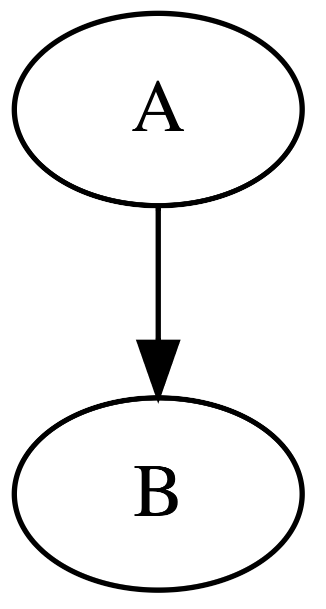
I would recommend using ‘png’ for the format. The final image renders to img/g2.png in this example. (Note that for our purposes we need to create nodes and edges from our own data structures.)
More graphviz examples here. For our application, create a directed graph in this style (with (k-1)-mers as the nodes) so the user can visualize the results.
Inside the DBG class you will also need methods for traversing the graph to create assemblies (in the form of contigs). Here are some suggestions (test each method on test1.fasta).
A method for determining if the graph is Eulerian. After you have built the de Bruijn graph, the first thing we will check is if it’s Eulerian. To do this, we need some way of determining the out-degree and in-degree of each node. However you decide to do this, you should have an Eulerian method that returns True if the graph is Eulerian (at most 2 semi-balanced nodes and all other nodes balanced) and False otherwise. Note that we are not considering different connected components of the graph (although you are welcome to create more nuanced methods that determine if each connected component is Eulerian on its own).
A method for finding semi-balanced nodes. More specifically, create a method that returns a list of nodes with (outdegree - indegree) = 1. These will form our start nodes and we’ll start each new path through the graph from one of these nodes.
A method(s) for traversing the graph. Create a method for traversing the graph, forming an Eulerian path (if possible). For the example datasets, the recursive algorithm discussed in class should be fine, but if you’re working on the (optional) genomeX dataset you will probably want to implement iterative path-finding. For this method we will need a stack to keep track of the path. In Python we can use lists as stacks, using append to add to the stack and pop to remove and return elements from the end. Note that traversing the graph will remove edges, thus destroying the graph. That is okay for this application. Your baseline traversal algorithm should have the start node (one of the semi-balanced nodes you found in the step above) and the path (which starts out empty) as arguments.
A method for finding all the contigs. You should now be able to start at each “start” node, traverse the path, and then find one contiguous sequence (contig). This can be done however you like (the loop over start nodes could be done in the DBG class or in main). Keep in mind the path is returned in reverse order (which is why we need to pop each node off to learn the sequence). Then write the contigs to a FASTA file.
You will define your main program in assembly.py. At a high level, your main should parse the command line arguments, build the DBG, then traverse it to create contigs, and finally write these contigs to a file.
Here are the specific details, but feel to add more functionality or print additional information along the way (in particular, you might want to print out the number of balanced and semi-balanced nodes).
Greet the user.
Create the de Bruijn graph with the given k value and print nodes/edges as shown above. This should be done by calling the __str__ method for the DBG using print(..).
Write the visualization (using graphviz) to a file with the prefix provided on the command line.
Determine if the graph is Eulerian and print True or False as shown above. You can also print out additional information like the number of balanced and semi-balanced nodes (optional).
Traverse the graph and find contigs, then write the contigs to a file in fasta format (as well as print them).
(Optional) Compute and print the N50 of the contigs.
There are 4 test files to practice on: test1.fasta, test2.fasta, test3.fasta, and genomeX_reads.fasta. Make sure the first 3 work, the fourth is optional (details below).
(Optional: genomeX_reads.fasta) For the fourth one, the reference (original) genome is provided as well: genomeX_reference.fasta. If you do run the fourth example, you can see how closely your assembly matches the original using the online tool BLAST and upload the two FASTA files. In the next few weeks we will see how to do this step (called sequence alignment) ourselves. It is okay if your assembly for this last test case has some issues, the coverage is good but not completely uniform. Experiment with k. In your README, explain which value of k produced the best assembly.
In addition to the requirements listed above, you should ensure your code satisfies these general guidelines (as well as the style guidelines linked on Piazza):
debruijn.py file.Make sure to fill out the README file as well as the results for the first three test cases. The files you should have at the end are (at a minimum):
README.mddebruijn.pyassembly.pyresults/test1.png and results/test1_contigs.fastaresults/test2.png and results/test2_contigs.fastaresults/test3.png and results/test3_contigs.fastaCreate a runtime plot
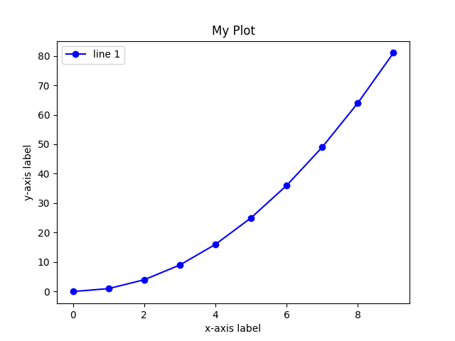
This extension ask you to analyze the runtime of building a de Bruijn graph. For this I would recommend using the genomeX reads and vary the number of reads you consider. Then plot the runtime as a function of the number of reads, in runtime.py. I will show the best runtime visualizations in class. Here is a rough sketch of how to use matplotlib for this purpose. I am happy to help get this working further.
import matplotlib.pyplot as plt
x = range(10)
y = [val**2 for val in x]
plt.plot(x,y,'bo-') # make sure x and y are the same length
plt.title("My Plot")
plt.xlabel("x-axis label")
plt.ylabel("y-axis label")
plt.legend(["line 1"])
plt.show()