The goals of this week's lab:
tensorflow and, optionally, keras)Note that there is a check in for this lab. By lab on April 10 you should have completed at least the data pre-processing (including flattening). Ideally you should have also started the fully connected neural network.
You must work with one lab partner for this lab. You may discuss high level ideas with any other group, but examining or sharing code is a violation of the department academic integrity policy.
Acknowledgements: adapted from Stanford CS231n course materials
To get started, find your git repo for this lab assignment in the cs66-s19 github organization.
Clone your git repo with the starting point files into your labs directory:
$ cd cs66/labs
$ git clone [the ssh url to your your repo]
Then cd into your lab07-id1_id2 subdirectory. You will have or create the following files:
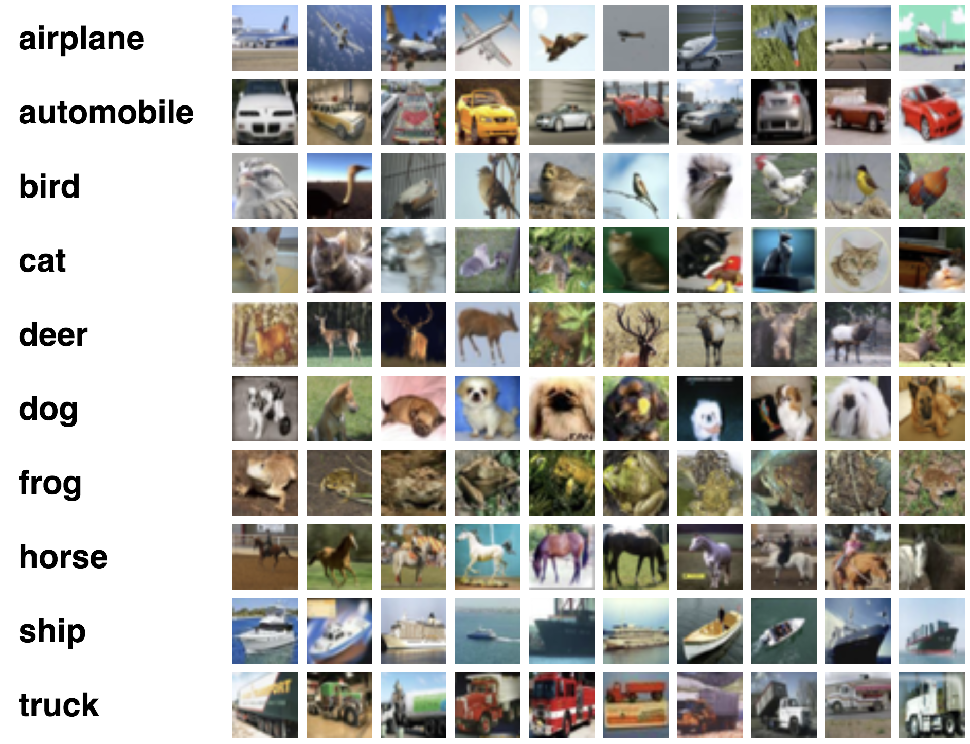
run_nn_tf.py - your main program executable training and testing NNs in base tensorflowfc_nn.py - implementation of a fully connected neural networkcnn.py - implementation of a convolutional neural networkrun_best.py - train and test your best neural network for the competition portionREADME.md - for analysis questions, results, and data collectionFor this lab, we will be investigating the CIFAR-10 dataset, which contains small images from 10 classes (examples shown below):
See Learning Multiple Layers of Features from Tiny Images by Alex Krizhevsky (2009) for more information about this dataset.
We will also be using a virtual environment for this lab (same one as AI since we will use some of the same libraries). Here is an example of how to enter the virtual environment, and how to exit when you are done:
$ source /usr/swat/bin/CS63env
$ <run python3 code as usual>
$ deactivate
Similar to Lab 6, we will be using high-level libraries, so consult the documentation frequently. Make sure you really understand each line of code you're writing and each method you're using - there are fewer lines of code for this lab, but each line is doing a lot!
When importing modules, avoid importing with the * - this imports everything in the library (and these functions can be confused with user-defined functions). Instead, import functions and classes directly. Imports should be sorted and grouped by type (for example, usually I group imports from python libraries vs. my own libraries).
For help with tensorflow, see the TensorFlow tutorials. Note that your final code will take a while to run, so please budget time for experimenting with different architectures.
1. First, examine the starter code in run_nn_tf.py. There are two global variables - the device controls whether or not we use a CPU vs. GPU. For this lab there is no need to use a GPU, but if you have access to a GPU and want to experiment, set this flag to True. The other variable, save_every will control how often we save the current training progress.
The Dataset class is a wrapper around a set of features/labels representing either train data, validation data, or test data. This allows us to iterate over the data in "mini-batches". In gradient descent, often we use only one data point at a time to update the model parameters. Here we will use mini-batches so that gradient updates are not performed quite so frequently (but also not as infrequently as if we had used the entire "batch"). Mini-batches are a middle ground between these two approaches.
You don't need to worry about combine_batches too much - this function reads the data in from a folder and combines data from different files. The load_cifar10 function allows you to choose the number of training, validation, and testing examples. Here, the input data X has 4 dimensions:
shape of X: (n, 32, 32, 3)where n is the number of examples. Each example is an image of size 32 x 32 pixels. Since we have RGB (red, blue, green) values for each pixel, the depth of the data is 3. We will also refer to 3 as the number of channels.
The first coding step is to modify the load_cifar10 function to subtract off the mean and divide by the standard deviation (normalize the data). This will make our data zero-centered and keep all the features roughly on the same scale (see image below).
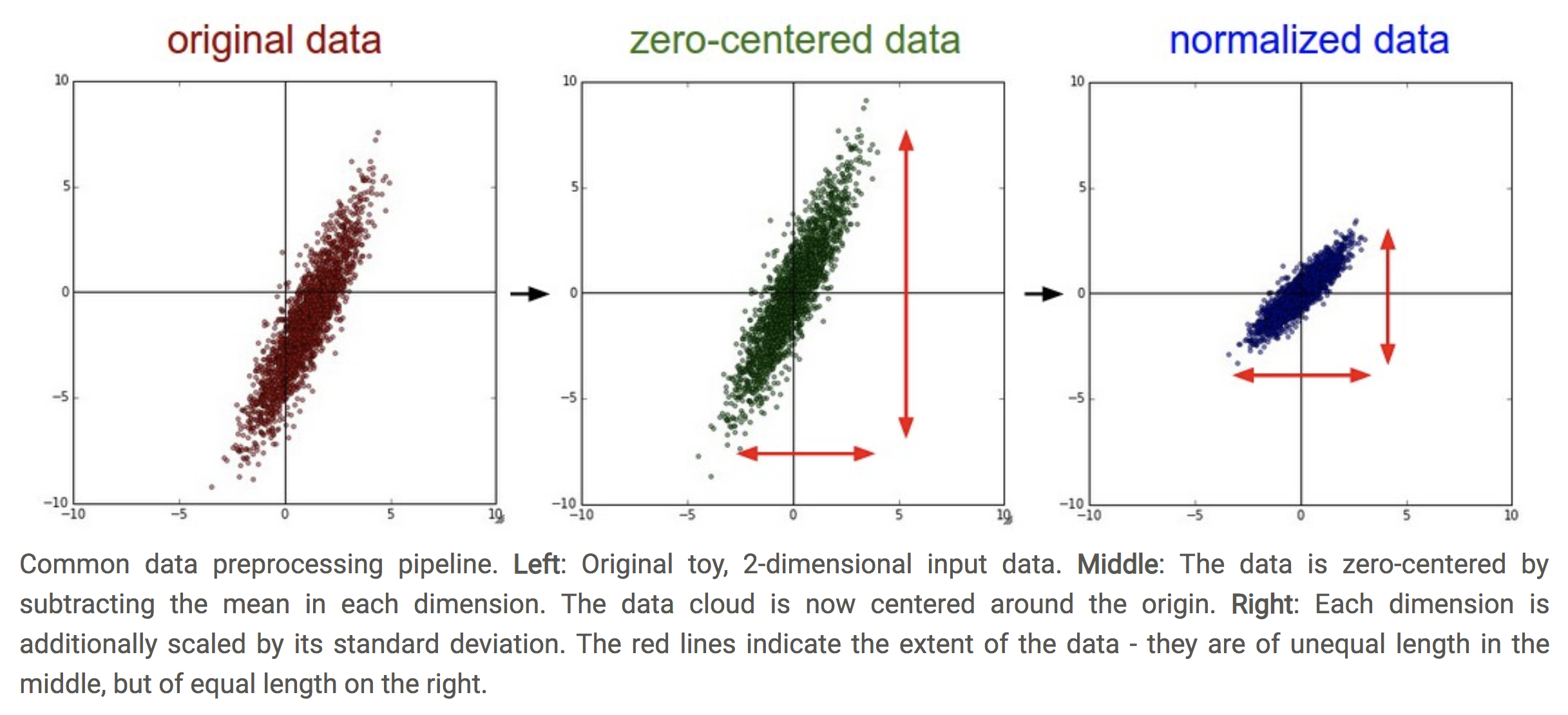
Figure from Stanford CS231n course, section "Neural Networks Part 2: Setting up the Data and the Loss"
We will compute the mean and std on the training data only, since we need to make sure to treat our validation and test data the same way we treated our training data (think back to the continuous feature transformation we did for Lab 2). To perform these operations on a matrix, you can use:
mean_pixel = dset.mean(axis=(0, 1, 2), keepdims=True)
std_pixel = dset.std(axis=(0, 1, 2), keepdims=True)
Where dset should now be the training data. We will compute the mean across the first 3 axes, but allow the RGB channels to have different means. keepdims=True allows the result to be broadcast into the shape of the original data. So after computing these matrices, subtract off the mean matrix and divide by the standard deviation matrix.
To test this part, run
python3 run_nn_tf.pyAnd make sure you get the dimensions for train, validation, and test as commented in the starter code.
train_dset, val_dset, and test_dset using the Dataset class. Here we will use a mini-batch size of 64. We will shuffle the train data, but not the validation and test data. To test this part, uncomment the iteration at the bottom of main and make sure that each mini-batch has size(64, 32, 32, 3)We are now ready to begin using the data to train neural networks.
3. In util.py, implement the flatten function. We will use this to "unravel" an image into a vector of pixels. We want to do this for all images at once, but we don't want to unravel them all together. So if we have 100 images, each of shape (32,32,3), we want to return a tensor of shape (100,32 * 32 * 3). See tf.reshape for more information (hint: what does the -1 do in reshape?)
We will make use of flatten in both our fully connected network and our convolutional network. But for the purposes of getting started, we'll test it in fc_nn.py:
python3 fc_nn.pyMake sure you get the same output described in the comments in main. This is the first example of running computations in tensorflow. These computations proceed in two phases:
Stage I: we set up a graph of tensors that have certain shapes, but we do not actually know any of the values of our data at this point.
Stage II: we feed data through this graph to perform computations. We usually set up a Session object and run the session by passing in data for some of our tensors, and requesting the computation of some unknown tensors. See the test_flatten function for an example. Make sure this idea makes at least some sense before moving on.
two_layer_fc. For a 2-layer network, we will have one hidden layer and two sets of weights (w1 connecting input to hidden layer, and w2 connecting hidden layer to outputs). More steps are provided in the starter code. We will use a ReLU non-linearity, but we will not apply this to the very last layer (we will let the loss function deal with making the outputs into a proper probability distribution).See references:
To test this part, again run fc_nn.py, and you should see a resulting shape of (64, 10). Make sure you understand what is going on in the function two_layer_fc_test (there is some explanation of each step).
python3 fc_nn.pytwo_layer_fc_init. Here we will have 4000 nodes in the hidden layer. For the initialization, we will use a Kaiming normal (more information in the starter code), which will allow us to take into account the number of inputs to each node. Here is an example of how to set up a tensorflow variable:w1 = tf.Variable(util.kaiming_normal(<shape>))
w2 = tf.Variable(util.kaiming_normal(<shape>))See tf.Variable for more information.
training_step function in run_nn_tf.py. This will perform one step of gradient descent (using one mini-batch of data) and update the weights.Now investigate the train function. This will be a flexible function we can use to learn any model_fn. Your task for this part is to complete the section that initializes the placeholders. First initialize x (4D tensor) and y (1D tensor). Since we won't know the mini-batch size in advance, you can put None for this part of the shape, then fill in the image size for the rest of the shape of x. Next, set up the params using the initialization function that was passed in, then set up the model and the loss (for the loss using the result of one training step).
Periodically we will check the accuracy on the validation dataset. We will not actually perform hyper-parameter turning here (although you are welcome to do that later), but the idea is that we will not use the testing data until the very end. We use this small validation set to check convergence. This accuracy check is performed using the check_accuracy function (read through this code as well).
main in run_nn_tf.py, call train and pass in the appropriate functions and parameters for a 2-layer fully connected network. Use a learning rate of:learning_rate = 3e-3Then run the code
python3 run_nn_tf.pyTo train the fully connected network on the training data. After one epoch (pass through all the training data), you should be able to get accuracies above 40%. We will return to the fully connected network later for comparison, but for now we turn to a different architecture.
cnn.py, we will set up the CNN architecture in the function three_layer_convnet. Our architecture will have two convolutional layers and one fully connected layer. Here is a summary:channel_1 filters, each with shape KW1 x KH1channel_2 filters, each with shape KW2 x KH2C classesFor now we will use strides=[1, 1, 1, 1] for the strides (meaning we shift the filter by "ones" in both the width and the height of the image) and padding='SAME', meaning zero padding.
See the documentation for tf.nn.conv2d, and there are more details about the shapes of the weights in the starter code. Run the function three_layer_convnet_test to confirm the shape of your result.
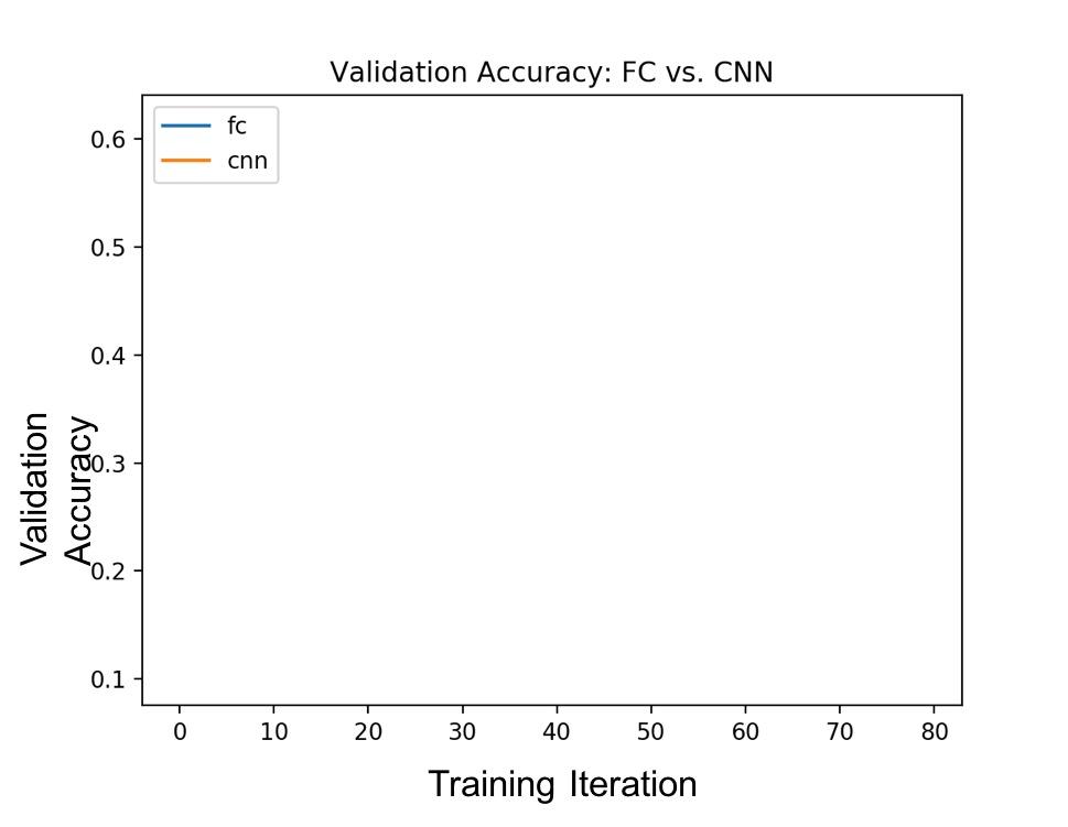
three_layer_convnet_init. For everything except the biases, we will use the Kaiming normal initialization. For the biases, we will initialize them to zeros. Here are the shapes to use:run_nn_tf.py, train a 3-layer neural network using the train function with the appropriate input functions and parameters. You can use the same learning rate. After one epoch you should be able to get over 43% accuracy.One common way to see how training is progressing is to plot accuracy against the training iteration (usually measured in terms of number of mini-batches processed). Right now we are only using one epoch (pass through the training data). Devise a way to increase the number of epochs to 10, and then create a plot of validation accuracy as a function of the training iteration, for both the fully connected NN and the CNN. Here is how the axes should be set up:
Also save the loss and create a plot of how it changes over the training iterations (for both methods). Here is how the axes should be set up:
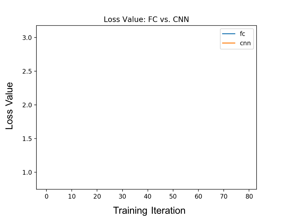
Include both images in your README, along with some brief analysis. Which method did better overall? Do you consider the networks to have converged after 10 epochs? If yes, at what point did they converge?
Devise a way to use your results to create a confusion matrix for the test data (which we so far have not used at all). Include these as either tables or images in your README (one matrix for each method). If you want to copy your results onto a visualization, you are welcome to download the figure below:
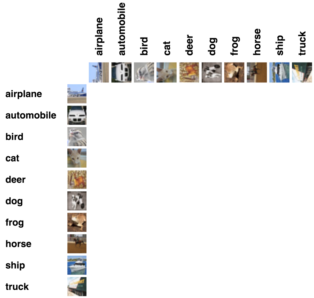
Include brief analysis about which classes seemed the most difficult.
In run_best.py, modify either your fully connected network or your CNN to increase the accuracy on the validation data as much as possible. Suggestions to try:
By the end of this part, you should have improved over the networks in the previous sections. Report your testing accuracy and testing confusion matrix in your README. You should be able to get at least 60-65% (edit to be a bit lower!) accuracy on the test data. Briefly discuss what you tried and what had the biggest impact in your README.
There will be a small prize for the group with the highest testing accuracy! Under the following conditions: you must create the network yourself. You may use keras if you prefer, but I must be able to run it with the CS63 virtual machine.
For the programming portion, be sure to commit your work often to prevent lost data. Only your final pushed solution will be graded. Only files in the main directory will be graded. Please double check all requirements; common errors include: