CS66 Lab 4: Probabilistic Models

Due: Friday, March 8 at 11:59pm

Overview

The goals of this week’s lab:

• Implement Logistic Regression
• Implement the Naive Bayes algorithm
• Handle multi-class prediction
• Understand the assumptions of both algorithms and how to compare them

You must work with one lab partner for this lab. You may discuss high level ideas with any other group, but examining or sharing code is a violation of the department academic integrity policy.

Note that there is a check point requirement for this lab; I will check that you have completed at least the Logistic Regression portion by lab on Wednesday, March 6 (but ideally you should have also made substantial progress on Naive Bayes!)

Getting Started

Find your git repo for this lab assignment in the cs66-s19 github organization.

Clone your git repo with the starting point files into your labs directory:

$ cd cs66/labs
$ git clone [the ssh url to your your repo]

Then cd into your lab04-id1_id2 subdirectory. You will have/create the following files:

• input - directory containing train/test data sets. You may add additional data sets here.
• outputLR - you should create this directory and save your Logistic Regression output here.
• outputNB - you should create this directory and save your Naive Bayes output here.
• run_LR.py - your main program executable for Logistic Regression.
• LogisticRegression.py - a class file to define your Logistic Regression algorithm.
• run_NB.py - your main program executable for Naive Bayes.
• NaiveBayes.py - a class file to define your Naive Bayes algorithm.
• README.md - for analysis questions and lab feedback.

Common Implementation Details

Usage

Your programs should take in 1 or 2 command-line arguments as in Lab 2. The first argument for both programs will be the data set. For logistic regression, you will also take in the learning rate for gradient descent (alpha). For example, to run Naive Bayes on the tennis example:

python3 run_NB.py tennis

If the user specifies an incorrect number of arguments, or invalid values for the parameters print a usage statement and exit the program. You should error check all parameters to ensure that the files exist. The learning rate must be greater than 0. E.g.,

$ python3 run_LR.py
Error, incorrect number of arguments
Usage: python3 run_LR.py dataset alpha
  dataset - base name of input files in the input/ folder
  alpha - learning rate during gradient descent

For logistic regression, the dataset will be in CSV (comma separate values) format. For Naive Bayes, the dataset will be in ARFF format. Note that the dataset name (e.g., tennis) will determine 3 file names:

• The training set file input/[dataset]_train.arff e.g., input/tennis_train.arff
• The test set file input/[dataset]_test.arff e.g., input/tennis_test.arff
• The predicted labels for the test set outputLR/[dataset].labels e.g., outputLR/tennis.labels. Save Naive Bayes output to the outputNB folder.

You must ensure that the two input files actually exist. Please follow this format exactly; these are easy points for your grade and they significantly reduce the number of issues during grading.

Program Inputs

To simplify preprocessing, you may assume the following:

• The data set will be in separate train and test files, as with Lab 2.
• Data will be in CSV format for logistic regression and ARFF format for Naive Bayes. You may either reuse your work from Lab 2 for parsing ARFF files or use any available library (e.g., scipy).
• You may assume that all features are discrete (binary or multi-class) and unordered. You do not need to handle continuous features, although you are welcome to reuse your thresholding code from Lab 2.
• Unlike Lab 2, prediction tasks can be multi-class (edit: just for Naive Bayes).
• You can and should reuse as much as you can from Lab 2 (e.g., checking command-line arguments, parsing input files, etc).

For Both Classifiers

• Your program should print a confusion matrix and accuracy of the result. Your program should also save the predicted labels (as with the previous project) in your output{NB,LR}/ folder.

• The design of your solution is largely up to you. At a minimum, each classifier should have a consistent public interface including a train(X,y) function which takes a set of training data (X and y) and a predict(x_new) function which returns a prediction for a test example (and, optionally, a predictAll(Xnew) method to loop over the entire test set).

• All pre-processing and post-processing should be done outside of the class definitions. You are welcome to create an additional library file for these types of functions. This could include a savePredictions function that works regardless of what method made the predictions as well as any parsers (e.g., readCSV, readARFF, etc) that returns the result of parsing input files. Your programs should minimize redundancy.

Part 1: Logistic Regression

You will implement the logistic regression task discussed in class for binary classification.

Model

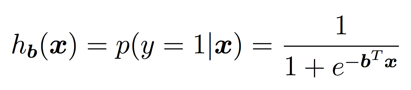
For now you should assume that the features will be continuous and the response will be a discrete, binary output. In the case of binary labels, the probability of a positive prediction is:

To model the intercept term, we will include a bias term. In practice, this is equivalent to adding a feature that is always “on”. For each instance in training and testing, append a 1 to the feature vector. Ensure that your logistic regression model has a weight for this feature that it can now learn in the same way it learns all other weights.

Training

To learn the weights, you will apply stochastic gradient descent as discussed in class until the cost function does not change in value (very much) for a given iteration. As a reminder, our cost function is the negative log of the likelihood function, which is:

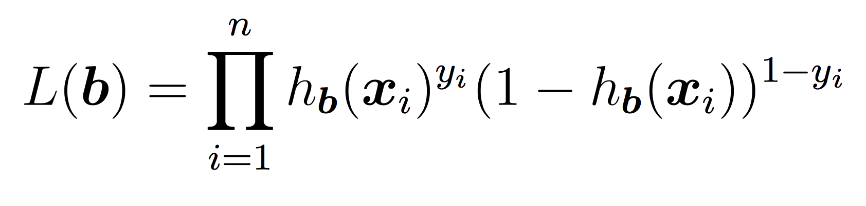
Our goal is to minimize the cost using SGD. We will use the same idea as in Lab 3 for linear regression. Pseudocode:

initialize weights to 0's
while not converged:
    shuffle the training examples
    for each training example xi:
        calculate derivative of cost with respect to xi
        weights = weights - alpha*derivative
    compute and store current cost

The SGD updates for each b_j term are:

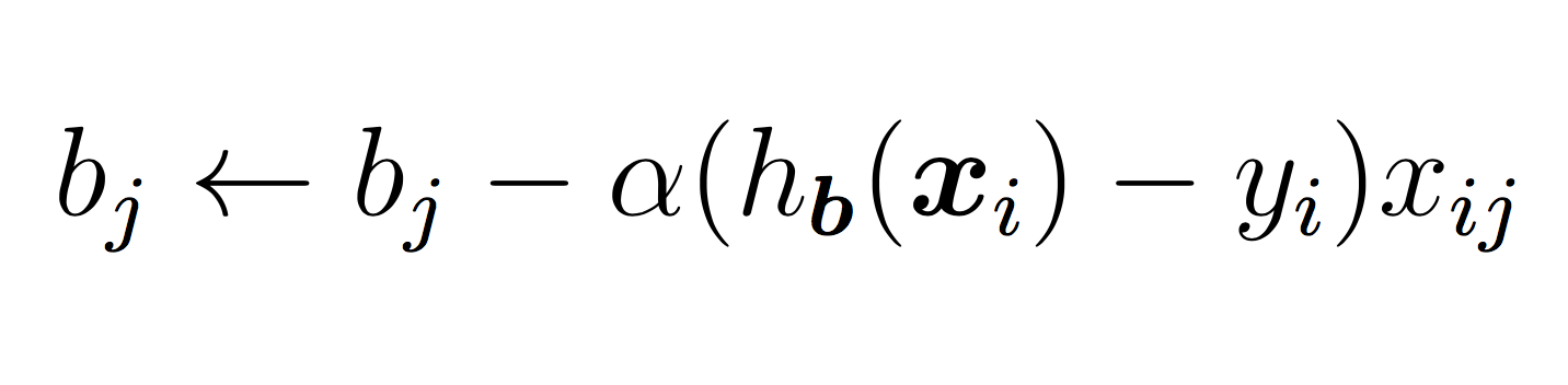
The hyper-parameter alpha (learning rate) should be sent as a parameter to the constructor and used in training. A few notes for the above:

• In Lab 3 we did not actually shuffle the data points to make gradient descent truly “stochastic”, but for this lab you should (also make sure y is shuffled along with X!). You may use:

numpy.random.shuffle(A)

which by default shuffles along the first axis.

• The stopping criteria should be a) a maximum of some number of iterations (your choice) OR b) the cost has changed by less some number between two iterations (your choice).

• Many of the operations above are on vectors. I strongly recommend using numpy features such as dot product to make the code simple.

• Try to choose hyper-parameters that maximize the testing accuracy.

Prediction

For binary prediction, apply the equation:

and output the more likely binary outcome. Use the Python math.exp function to make the calculation in the denominator.

The choice of hyper-parameters will affect the results, but you should be able to obtain at least 90% accuracy on the testing data. Make sure to print a confusion matrix and output a file of predicted labels.

Example Output

Here is an example run for testing purposes. You should be able to get a better result than this, but this will check if your algorithm is working. The details are:

• No shuffling of the training data points (which you should do for the final result!)
• alpha = 0.02
• stopping criteria: looking for changes in the cost J(b)
• epsilon = 1e-4 (see if cost has changed by this amount)

$ python3 run_LR.py phoneme 0.02
Accuracy: 0.875000 (70 out of 80 correct)

   prediction
      0  1
    ------
  0| 36  4
  1|  6 34

Labels and Debugging Output

Part 2: Naive Bayes

You will implement Naive Bayes as discussed in class. Your model will be capable of making multi-class predictions.

Model

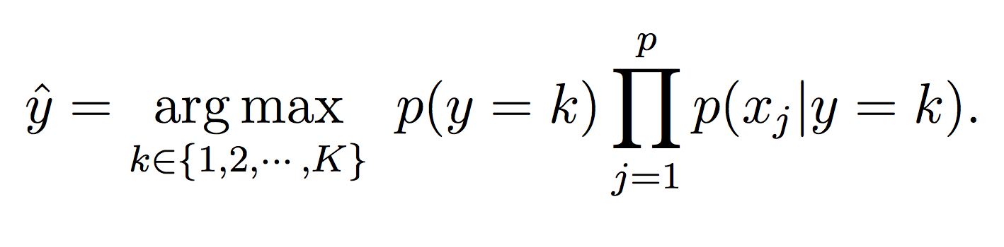
Recall that our Naive Bayes model for the class label k is:

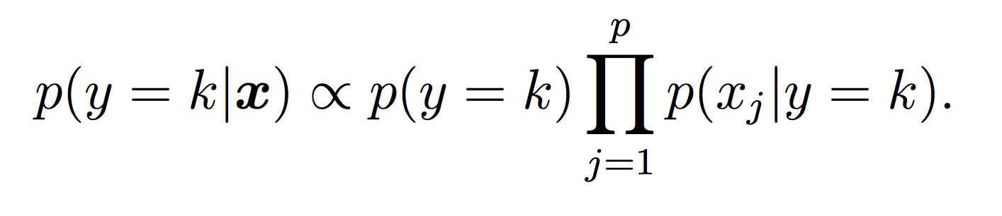
For this lab, all probabilities should be modeled using log probabilities to avoid underflow. Note that when taking the log of a formula, all multiplications become additions and division become subtractions. First compute the log of the Naive Bayes model to make sure this makes sense.

Training

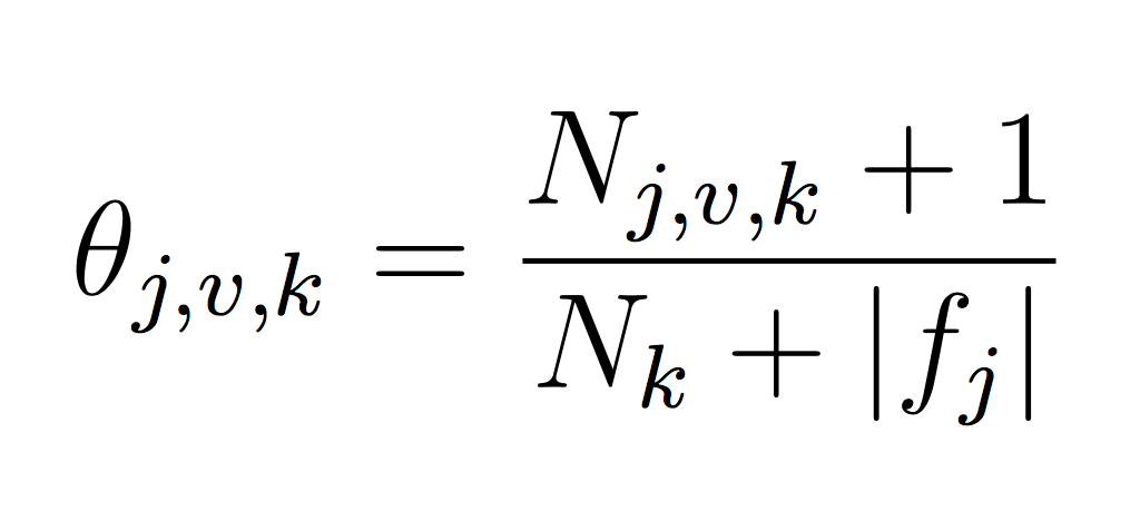
You will need to represent model parameters (θ’s) for each class probability p(y = k) and each class conditional probability p(x_j = v|y = k). This will require you to count the frequency of each event in your training data set. Use LaPlace estimates to avoid 0 counts. If you think about the formula carefully, you will note that we can implement our training phase using only integers to keep track of counts (and no division!). Each theta is just a normalized frequency where we count how many examples where x_j = v and the label is k and divide by the total number of examples where the label is k (plus the LaPlace estimate):

And similarly for the class probability estimates:

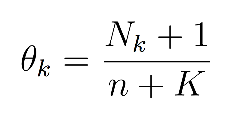
If we take the log then each theta becomes the difference between the two counts. The important point is that it is completely possible to train your Naive Bayes with only integers (the counts, N). You don’t need to calculate log scores until prediction time. This will make debugging (and training) much simpler.

Inference/Prediction

For this phase, simply calculate the probability of each class (using the model equations above) and choose the maximum probability:

Example Output

• Tennis example:

$python3 run_NB.py tennis
Accuracy: 0.928571 (13 out of 14 correct)

  prediction
     0  1
   ------
 0|  4  1
 1|  0  9

Labels and Debugging Output

• Zoo example:

$python3 run_NB.py zoo
Accuracy: 0.857143 (30 out of 35 correct)

        prediction
     0  1  2  3  4  5  6
   ---------------------
 0| 13  0  0  1  0  0  0
 1|  0  7  0  0  0  0  0
 2|  0  1  0  0  1  0  0
 3|  0  0  0  4  0  0  0
 4|  0  0  0  0  1  0  0
 5|  0  0  0  0  0  3  0
 6|  0  0  0  0  0  2  2

Labels and Debugging Output

Part 3: Analysis and Comparison

(See README.md to answer some of these questions)

So far, we have run logistic regression and Naive Bayes on different types of datasets. Why is that? For the analysis portion, explain how you could transform the CSV dataset with continuous features to work for Naive Bayes. Then explain how you could transform the ARFF datasets to work with logistic regression.

Finally, implement one of your suggestions so that you can properly compare these two algorithms. One concrete suggestion: either create a method that will convert ARFF to CSV, or visa versa. You will have to transform some of the features (and possibly outputs) along the way, but that way you won’t have to modify your algorithms directly.

For making logistic regression work in the multi-class setting, you have two options. You can use the likelihood function presented in class and run SGD. Or you can create K separate binary classifiers that separate the data into class k and all the other classes. Then choose the prediction with the highest probability.

Extensions

1. The analysis portion only requires you to make one algorithm work for both types of datasets. Implement both ways so that both algorithms can work on both datasets.

2. Create a visualization of logistic regression for the “phoneme” dataset. One idea for this is to use PCA (principal components analysis) to transform X into a single feature that can be plotted along with y.

Submitting your work

For the programming portion, be sure to commit your work often to prevent lost data. Only your final pushed solution will be graded. Only files in the main directory will be graded. Please double check all requirements; common errors include:

• Did you fill out the README?
• Did you remove all debugging/developer comments including TODOs and print statements?
• Are all functions and non-trivial portions of code commented and easy to follow?
• Recheck your code on a lab machine to make sure it runs. Students often have whitespace errors are doing a last past of adding/removing comments.

Acknowledgements

Credit for this lab: modified from material created by Ameet Soni. Phoneme dataset and information created by Jessica Wu.

Information about the datasets:

• The task of phoneme classification is to predict the phoneme label of a phoneme articulation given its corresponding voice signal. In this problem, we have voice signals from two different phonemes: “aa” (as in “bot”) and “ae” (as in “bat”). They are from an acoustic-phonetic corpus called TIMIT.

• Zoo data from Zoo Animal Classification by Kaggle. The class labels are: