CS66 Lab 2: Decision Trees

Due: Tuesday, February 12 Thursday, February 14 at 11:59pm

Overview

The goals of this week’s lab:

• Implement the decision-tree algorithm
• Handle common data-processing tasks including file parsing and feature conversion
• Implement schemes to prevent overfitting
• Perform experimental analysis on your decision tree

You must work with one lab partner for this lab. You may discuss high level ideas with any other group, but examining or sharing code is a violation of the department academic integrity policy.

Note that I will not be in lab January 30, but I still strongly recommend that you begin in lab with your partner. During lab on Feb 6, I will go around to each group for an intermediate “check-off”. At that point you should have at least designed your data structures and implemented a top-down design for your entire program (and have both partners be able to explain it to me!)

Getting Started

Find your git repo for this lab assignment in the cs66-s19 github organization.

Clone your git repo with the starting point files into your labs directory:

$ cd cs66/labs
$ git clone [the ssh url to your your repo]

Then cd into your lab02-id1_id2 subdirectory. You will have the following files:

• input - directory containing train/test data sets including the heart and diabetes data sets. You may add additional data sets here.
• output - all required output from your algorithm should be saved here
• run_dtree.py - your main program executable
• DecisionTree.py - a class file to define your decision tree algorithm
• README.md - for analysis questions and lab feedback

Part 1: Implement a Decision Tree

You will implement an ID3-like decision tree in this part of the lab. The main features of your implementation include:

• Reading in ARFF formatted train and test set files
• Converting continuous features into thresholded binary features
• Building trees to a maximum depth as determined by user input
• Output of learned tree for interpretation of induced model
• Evaluation of the constructed tree on a held-aside test set

Usage

Your program should take in 1 or 2 command-line arguments in this specific order:

1. The name of the data set
2. A parameter setting for the maximum depth of the learned tree (optional)

For example:

python3 run_dtree.py heart 3

If the user specifies an incorrect number of arguments, or invalid values for the parameters print a usage statement and exit the program. You should error check all parameters to ensure that the files exist and that given parameters are integers greater than 0. E.g.,

$ python3 run_dtree.py
Error, incorrect number of arguments
Usage: python run_dtree.py dataset [depth]
  dataset - base name of input arff files in the input/ folder
  depth (optional) - maximum depth of tree, set as a positive integer value

Note that the dataset name (e.g., toy) will determine 4 file names:

• The training set file input/[dataset]_train.arff e.g., input/toy_train.arff

• The test set file input/[dataset]_test.arff e.g., input/toy_test.arff

• The tree output file output/[dataset].tree e.g., output/toy.tree

• The predicted labels for the test set output/[dataset].labels e.g., output/toy.labels

You must ensure that the two input files actually exist. Please follow this format exactly; these are easy points for your grade and they significantly reduce grading issues.

Program Style Requirements

• Your program should follow good design practices - effective top-down design, modularity, commenting for functions and non-trivial code, etc.
• You should break your program up into multiple files with run_dtree.py as the main executable. You should build classes in separate files (I have provided one, you may add others). At a minimum, you should represent decision nodes and the decision tree as objects. Be sure to design these aspects of the program first before starting your main implementation.
• All decision tree algorithm details should be encapsulated in your decision tree class. The main file should only directly handle data parsing and the main control flow for calling decision tree steps (e.g., train, test, output).
• Practice defensive programming; e.g., did the user provide enough arguments on the command line? Do the files exist? You do not need to check if the contents are correct.
• Do not interact with the user for your program - if an incorrect filename is given, simply exit the program with a message; do not prompt for a new file.
• Clean up any debugging print statements at final submission. It may be useful to use these during development, but need to be cleaned up before we grade them.
• All functions should include a top-level comment describing purpose, parameters, and return values.
• Avoid using existing libraries to solve major components of the program. For example, I want you to manually parse the ARFF files instead of using an ARFF library that exists. You are more than welcome to use numpy for array management. Please ask me if there are other libraries you are interested in using.

Program Inputs

• Your program is expected to read files that are in the ARFF format. You are required to defend against non-existent files, but if you are given a valid file name, you can assume that it is in ARFF format.

• The header of the file describes the features and class label. You can assume that the class label is the last line in the feature list and will be named class to easily demarcate the end of the header. You can also assume the headers in the train and test files are the same.

• Subsequent lines after the header contain one example per line represented as commas separated feature values. The feature values occur in the same ordering as feature descriptions in the header (with the class label being at the end of the line).

• Your program should handle both discrete and continuous features. You can assume the class label is discrete.

• Lines starting with % are comments and should be ignored.

• I have provided data sets for testing purposes in the input directory including a heart disease prediction task (heart_{train,test}.arff) and a diabetes prediction task (diabetes_{train,test}.arff). You are encouraged to add your own toy examples for the purposes of debugging. Be sure to follow the format required in the usage.

• The other type of input is the optional maximum depth of the tree. This should be a positive integer - all other values (including 0) should be rejected and lead to a clean exit with error message. E.g., a depth of 1 means there is a single decision node in the tree. If no value is given, trees should be built using the same criteria as ID3.

Program Main Behavior

Your program should process inputs, parse and index training and test examples, and induce a decision tree. There are very few restrictions on how you do this, but be sure your tree fits the behavior from class:

• Never use information from the test set in any part of learning the tree, including when you decide thresholds for continuous features.

• You may assume that the prediction task is binary (use the values given in the header file). You can implement multi-valued prediction as an extension (see below).

• Continuous features should be converted into multiple binary features using thresholding at class label changes. The feature should use the less than or equals to relation (i.e., the feature is true if a feature value is <= to the threshold). Choose the mid-point between two adjacent feature values. E.g., if there is a label change from X=20 and X=30, you should add a feature X<=25.

• There should be a branch for each discrete value of a variable. This is described in the header of the arff file, and is limited to true and false for the converted continuous features. It is probably simplest to store these as string type.

• Use information gain for your selection criteria. You can break ties arbitrarily.

• The stopping criteria for a leaf is:

  • All examples are the same label.
  • There are no features remaining to split on.
  • The maximum depth of the branch has been reached.
  • No features produce information gain.

  The labels at leaves should be the plurality label of the examples at the leaf (in other words, we will not use probabilities for predictions). Ties can be broken arbitrarily.

Program output

When run, your program should output the following:

• To standard output, only print out the overall accuracy of the tree on the test set e.g.,

Accuracy: 0.70 (35 out of 50 correct)

• A formatted decision tree in output/[dataset].tree to visualize the learned model. See example outputs below for formatting help. In general, you will print the tree in pre-order traversal (print the current node, recurse on the left node, then recurse on the right node) with each node having one line of output for each branching child. The line should be tabbed based on the current depth, then include the name of the feature/feature-value pair, and the distribution of class labels for examples that reached that node. If you have reached a leaf, also append the label that would be returned.

  For example, here is the result of the PlayTennis concept from Handout 1 (note that the ordering of branches is irrelevant). At the root, there are 9 days tennis is played and 5 days it is not.

[9 5]
Outlook=Sunny [2 3]
|   Humidity=High [0 3]: No
|   Humidity=Normal [2 0]: Yes
Outlook=Overcast [4 0]: Yes
Outlook=Rain [3 2]
|   Wind=Strong [0 2]: No
|   Wind=Weak [3 0]: Yes

• A file with the predicted labels from the test set. The labels should output one per line, in the same order as the example originally appeared in the test file. Only print the predicted label, not the true label.

Example runs

Heart disease data set:

• No depth: Tree, Labels, 72 out of 103 correct
• Depth=5: Tree, Labels, 74 out of 103 correct
• Depth=1: Tree, Labels, 75 out of 103 correct

Diabetes data set:

• No depth: Tree, Labels, 67 out of 100 correct
• Depth=5: Tree, Labels, 69 out of 100 correct
• Depth=1: Tree, Labels, 68 out of 100 correct

Part 2: Analysis

UPDATE: the plotting part is now optional (you should still run various depths for both datasets and include your observations in your README, but you don’t need to make a plot).

Once your lab is complete, generate two learning curve graphs (i.e., line graphs) with an accompanying analysis of the graphs. On the x-axis, show the depth of a tree. On the y-axis, show the accuracy of the tree on both the training set and test set. Run experiments at various depth levels including, at a minimum, depths of 1, 2, 4, 7, and 10. You should have one graph for the diabetes data set and one graph for the heart disease data set.

Describe what you can conclude from each graph. What happens to the training set accuracy and test set accuracy as the depth varies? Is this what you expected? Place your graphs and analysis in the README.md. Be sure that your graphs are of scientific quality - including captions, axis labels, distinguishable curves, and legible font sizes. You can include a figure in Markdown using:

![Figure title](figure.png)

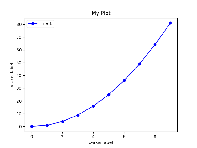
Here is an example of creating a plot using matplotlib, but you are welcome to use a different program for this part.

# import plotting library
import matplotlib.pyplot as plt

# set up sequences of x and y values (make sure they are of the same length)
x = range(10)
y = [val**2 for val in x]

# plot the (x,y) values (considered as pairs), using blue (b) circles (o),
# connected by lines (-)
plt.plot(x,y,'bo-')

# title, axis labels, and legend
plt.title("My Plot")
plt.xlabel("x-axis label")
plt.ylabel("y-axis label")
plt.legend(["line 1"])

# I usually use "show" at first to see the plot, then save it later
plt.show()
#plt.savefig("my_plot.png", format='png')

Extensions (Optional)

Multi-class prediction

Both data sets I have provided have two class labels. Decision trees easily extend to multi-class prediction. Find a relevant data set (e.g., at Kaggle or the UC Irvine Machine Learning Repository) and evaluate your algorithm with multiple discrete values allowed for labels.

Min Leaf Size

Another approach to prevent overfitting is setting a minimum number of examples in a leaf. If a split causes results in children below the threshold, the recursion is stopped at the current node and a leaf is created with the plurality label. This is often more flexible than maximum depth - it allows variable depth branches while still trying to prevent overly detailed hypotheses that only fit to a few examples. Add minimum leaf size as an optional command line argument.

Learning curves for training set size

Machine learning algorithms are often sensitive to the amount of training data - some algorithms thrive when there is large amounts of data but struggle when data is sparse (e.g., deep neural networks) while others plateau in performance even if more data is available. Evaluate your decision tree on the given training data by randomly subsampling the data to create smaller training sets e.g., use 10% of training data. Choose at least 5 training set sizes and plot them on the x-axis with the y-axis describing the accuracy. You’ll probably want to run each training set size 3-5 times and average the results. Describe what you see when you compare training and test accuracy as the training set grows.

Submitting your work

For the programming portion, be sure to commit your work often to prevent lost data. Only your final pushed solution will be graded. Only files in the main directory will be graded. Please double check all requirements; common errors include:

• Did you fill out the README?
• Did you remove all debugging/developer comments including TODOs and print statements?
• Are all functions and non-trivial portions of code commented and easy to follow?
• Recheck your code on a lab machine to make sure it runs. Students often have whitespace errors are doing a last past of adding/removing comments.

Acknowledgements

Credit for this lab: Ameet Soni.

Both data sets were made available by the UC Irvine Machine Learning Repository. The heart disease data set is the result of a study by the Cleveland Clinic to study coronary heart disease. The patients were identified as having or not having heart disease and the resulting feature set is a subset of the original 76 factors that were studied. The diabetes data set is the result of a study of females at least 21 years old of Pima Indian heritage to understand risk factors of diabetes. Both data sets were converted to ARFF format by Mark Craven at the University of Wisconsin.