Credit for this lab: Yun S. Song and Andrew H. Chan
Note the due date, this is a 1.5 week lab. This is the last graded lab, and the second midterm will be on Thursday April 19.
The goals of this lab are:
Find your partner and clone your lab08 git repo as usual. You should see following starter files:
README.md - questionnaire to be completed for your final submissionhmm.py - top-level file where you should read in the data, run your different algorithms, and output the resultsviterbi.py - where you should implement the Viterbi algorithmbaum_welch.py - where you should implement the forward-backward algorithm (and in Part 2, the training portion)example/ - directory with example data and example output filesdata/ - directory with input dataIn hmm.py I have written some code to parse the initial parameter file and create such a file after parameter estimation.
You are also welcome to add additional python files as long as the top-level files are the same. There are also a lot of command-line arguments, so feel free to create a script to run the top-level file.
See Durbin Chapter 3 and notes from Days 25-29 (we'll need class on Friday for Part 2).
In this lab we will consider the problem of finding the coalescence times for two sequences (i.e. a single individual). This problem can be formulated as an HMM (see Slides 28 for more details). Our observations will take on 2 values (i.e. B=2). We will encode the observation as a 0 if the two sequences are the same at a single base, and 1 if they are different. The length of this observed sequence is L=100kb.
The hidden state will be the coalescence time of the two sequences (i.e. the Tmrca for a sample of size n=2). For simplicity, we will discretize time into 4 states, represented by the times:
TIMES = [0.32, 1.75, 4.54, 9.40] # in coalescent unitsIn terms of how we will encode the states in the HMM, we will represent these states by their index (i.e. 0,1,2,3). This means that K=4 (number of hidden states).
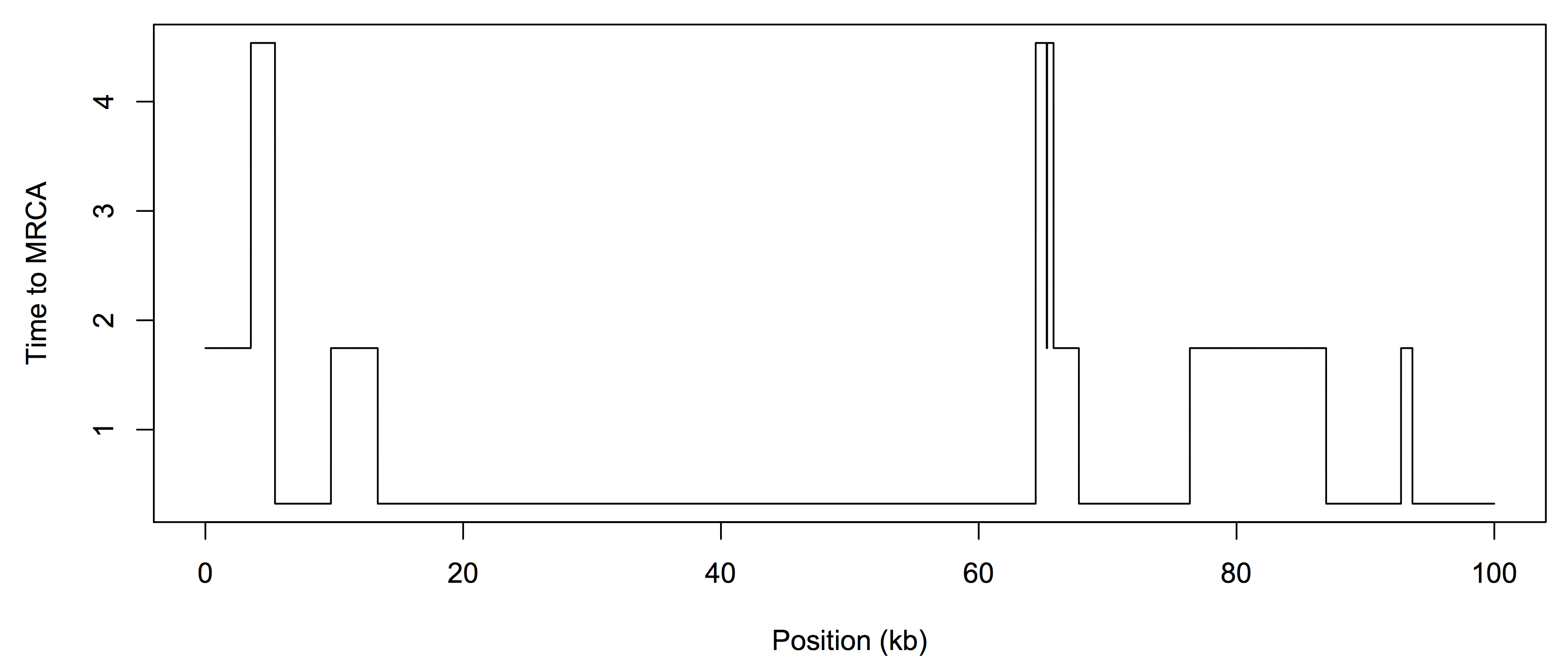
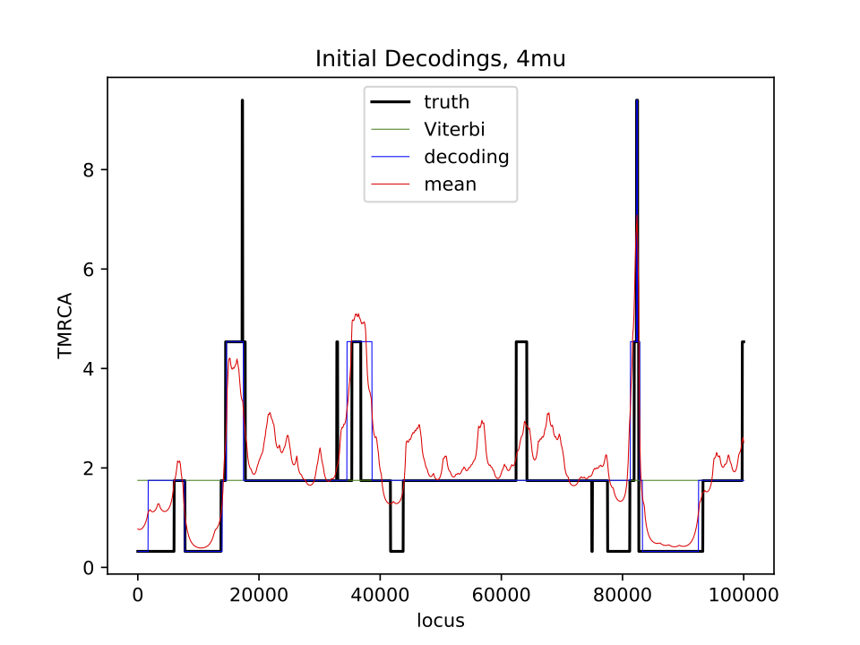
The observed data is in fasta format, i.e. sequences_4mu.fasta. The "mu" value represents the mutation rate, so we will investigate how changing the mutation rate affects our ability to determine the coalescence times. There are two sequences in each fasta file, and you should reduce them to a single sequence of 0s (same) and 1s (different). The data was generated under a ground "truth" - the true Tmrca of the two sequences. We do not know this ahead of time, but we will use it to see how closely we can estimate the hidden state sequence. Here is an example of the Tmrca along the genome, for n=2:
The initial parameters for the example are in the file initial_parameters_4mu.txt:
# Initial Probabilities
# k P(z_1 = k)
  0  0.603154
  1  0.357419
  2  0.0388879
  3  0.000539295


# Transition Probabilities
# a_{kl}, k = row index, l = column index
#    0               1               2              3
0.999916    0.0000760902    8.27877e-6  1.14809e-7
0.000128404 0.999786    0.0000848889    1.17723e-6
0.000128404 0.000780214 0.999068    0.0000235507
0.000128404 0.000780214 0.00169821  0.997393


# Emission Probabilities
# k  P(0|z=k)  P(1|z=k)
  0 0.999608 0.000391695
  1 0.998334 0.00166636
  2 0.995844 0.00415567
  3 0.991548 0.008452
This file shows the probability of starting in each state, the probabilities of transitioning between states (Markov chain "backbone"), and the probabilities of emitting a 0 or 1 based on the hidden state.
I would recommend the following command-line arguments, although for this lab I am open to you defining your own or modifying these a bit:
$ python3 hmm.py -f example/sequences_4mu.fasta -p example/initial_parameters_4mu.txt
-t example/true_tmrca_test.txt -i 15 -o example/ -s 4muThere is no specific terminal output you need to produce (whatever would be helpful for you). Most of the output will be done through writing files and creating plots.
First, implement the Viterbi algorithm in viterbi.py. The input to this function (or class) should be the observed sequence and a set of parameters (for now we will use the provided initial parameters, but make sure your function is general). You are welcome to store the parameters however you like (you could make a class for them, or a tuple of 3 numpy arrays, etc).
Your Viterbi function should return the most probable path (i.e. a sequence of the numbers 0,1,2,3) that is the length of the observed sequence. For the initialization, use the initial probabilities, not a special start state (see Slides 28).
Make sure to work in log-space! (Discussed in lab) Otherwise, underflow errors are very likely when multiplying together many small probabilities. See the Output section to check your results.
Second, implement the Forward algorithm in the file baum_welch.py. This should have the same input as the Viterbi algorithm. Instead of a best path though, I would recommend returning the entire forward table, since we will need to combine it with the backward values to get the posterior decoding. Make sure to again work in log-space.
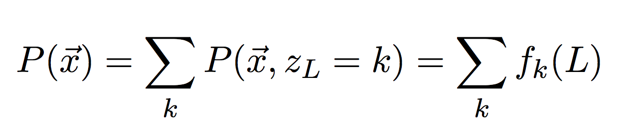
To check your forward-algorithm, add up the last column to get the total probability of our observed sequence. In log-space, this is referred to as the log likelihood.
Then compare your answer to the first number in the output file likelihoods_4mu.txt. You should get:
initial log-likelihood: -1612.708950Then implement the Backward algorithm in a separate function (same inputs as Viterbi and Forward), and again return the entire backward table.
Once you have the forward and backward algorithms working, we will put them together to compute the posterior probability (i.e. the probability given the observations) of observing each state at each time step. Create a table of the same size as your forward and backward tables, and fill it in with the posterior probabilities (first equation below).
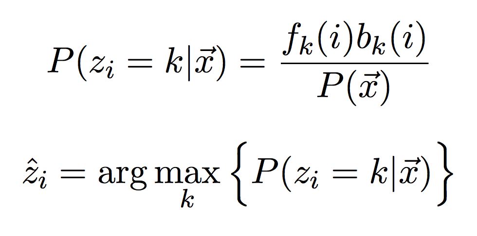
Then for each column, select the state with the highest value (second equation above). This is the posterior decoding or just "decoding" for short. This is what we can compare to the Viterbi path! It is not a path since we looked at each step separately and made a decision about the hidden state separately, but taken together it does form a hidden state sequence.
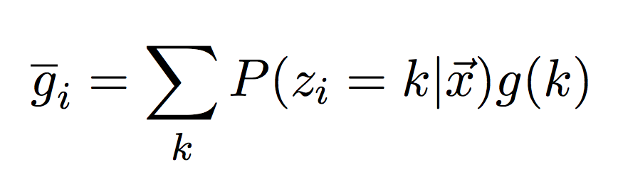
Instead of taking just the max, we can also take the average or what we call the posterior mean (or just mean for short). In this case, we don't just want to take the average of the values in each column, we want to take their average, weighted by the true value they represent. Let g(k) be a function that maps the hidden state index to its actual time value (shown above). I.e. g(2) = 4.54. We can compute the posterior mean by weighting each actual time value by its posterior probability.
In summary, between Viterbi and the forward-backward algorithms, we have 3 ways of estimating the hidden state. The output section below shows how to return and plot them to get a comparison image.
For each dataset you should produce 6 output files. Only 3 are relevant for Part 1. I'm showing the ones for 4mu here, but for the other datasets they should be similarly labeled.
decodings_initial_4mu.txt: this should be a Lx3 matrix showing each step and the estimated hidden time value. Here is the beginning of this file:# Viterbi_decoding posterior_decoding posterior_mean
1.75 0.32 0.772645
1.75 0.32 0.772550
1.75 0.32 0.772455
1.75 0.32 0.772360
1.75 0.32 0.772266
1.75 0.32 0.772172
1.75 0.32 0.772079
1.75 0.32 0.771986
...(Part 2) decodings_estimated_4mu.txt: the same format as for the initial parameters, but now after we have estimated the parameters (after Part 2).
(Part 1 and Part 2) likelihoods_4mu.txt: this file should only have two values, the initial log-likelihood (Part 1) and the final log-likelihood (Part 2).
(Part 1) plot_initial_4mu.pdf: a plot showing the true Tmrca and the 3 estimated hidden time sequences.
(Part 2) plot_estimated_4mu.pdf: the same as for the initial, but after parameter estimation (not included in starter files).
(Part 2) estimated_parameters_4mu.txt: estimated parameters (after Part 2).
In the second part of the lab, we will assume the initial parameters are a guess, and we will try to work towards the parameters that maximize the log-likelihood. (Note: we will need class on Friday for this part). Using the Baum-Welch algorithm, we will iterate between running the forward-backward algorithm and updating our parameters. These updates are given in Equations 3.18-3.21.
The output below shows Baum-Welch run for 15 iterations (recommended) with the log-likelihood shown for each iteration. Often will will want to run until the log-likelihood is not changing very much, but in this case 15 iterations is fine. This will take some time (minutes, not hours).
$ python3 hmm.py -f example/sequences_4mu.fasta -p example/initial_parameters_4mu.txt
    -t example/true_tmrca_test.txt -i 15 -o example/ -s 4mu
Baum-Welch
Iteration: 0
-1612.7089501433543
Iteration: 1
-1599.8947193372312
Iteration: 2
-1597.919646650623
Iteration: 3
-1597.1002683828203
Iteration: 4
-1596.6948497163282
Iteration: 5
-1596.418574853555
Iteration: 6
-1596.2027645959113
Iteration: 7
-1596.0224085370764
Iteration: 8
-1595.8676710371346
Iteration: 9
-1595.7352759554544
Iteration: 10
-1595.624410825711
Iteration: 11
-1595.5346251019898
Iteration: 12
-1595.4647793374975
Iteration: 13
-1595.4127166365138
Iteration: 14
-1595.3754719265296
Iteration: 15
-1595.3497675302026
At the end of this training process, we will have new estimated parameters. Given these parameters, run through the algorithms from Part 1 again to obtain estimated hidden time sequences, an estimated plot, and the final likelihood. I would recommend putting this training in baum_welch.py since it relies on the forward-backward algorithm.
Try to have your variable names match our class notation as much as possible, and always note when a variable is in log space (i.e. log_emit for emission probabilities).
Create some checks to ensure that your probabilities sum to 1 (or 0 in log-space). They will probably not sum to 1 exactly, but should be within 10e-6 of 0 in log-space.
What happens if you start with different initial parameters and/or run the training for more iterations? Feel free to submit additional parameter files and output files (in a separate folder). It would also be interesting to plot the log-likelihood against the iteration to see how it changes during training.
Make sure to push your code often, only the final version will be submitted. The README.md file asks a few questions about your results. Answer these questions and make sure to push the following files.
README.mdhmm.pyviterbi.pybaum_welch.pyexample/plot_estimated_4mu.pdf (for the example dataset)