
This lab again has 3 parts, which will be weighted roughly equally:
The goals of this lab are:
Find your partner and clone your lab07 git repo as usual. You should see following starter files:
README.md - questionnaire to be completed for your final submissioncoal_sims.py - where you should implement coalescent experimentsreal_data.py - where you should analyze the real data (1000 genomes data)In real_data.py I have written the beginning of a VCF file parser for the real data. You are welcome to modify this or write your own.
You are also welcome to add additional python files as long as the top-level files are the same.
The first part of the lab is a short tutorial on msprime and a set of experiments to test the theory we have developed in class. I would describe this part as more scripting and less as a program that someone else will use and modify. The goal is to understand coalescent expectations and observe them in practice.
msprime is a fast coalescent simulator, meaning that it creates synthetic SNP data using the coalescent as an evolutionary model. msprime is a python-based reimplementation of Hudson's original ms coalescent simulator. To use it, we will need to use the virtual machine that Jeff set up for our class:
$ source /usr/swat/bin/CS683env
# run python code (using msprime) as usual
$ deactivateHere are a few examples of how to use msprime based on the tutorial. Try out these examples to make sure the parameters and output make sense.
n=5 sequences and population size N=1000. In the manual this is referred to as the effective population size - for the purposes of this class we can think of effective population size as the fraction of samples that contribute genetic material to the next generation. It is related to the true population size but the relationship is complicated and for now we will think of these two quantities as describing the same idea.In this example there is no recombination, so there is only one tree, which should look different for you than my example below.
>>> import msprime
>>> tree_sequence = msprime.simulate(sample_size=5, Ne=1000)
>>> tree = tree_sequence.first()
>>> print(tree.draw(format="unicode"))
To analyze past evolutionary events, we will compute the branch lengths of this tree. In class we developed a theory of what we expect from these branch lengths, so now we will see if the reality matches our expectation. msprime makes these lengths very accessible. Somewhat confusingly, the nodes of the tree are integers, with 0,1,...(n-1) representing our sample, and increasing integers used as the internal nodes.
msprime allows us to see the time of a node and the branch length connecting the node to its parent. We can also ask for the parent of a node. Here are two examples for node 3 and node 5:
>>> tree.time(3)
0.0
>>> tree.branch_length(3)
672.5545584887533
>>> tree.parent(3)
6
>>>
>>> tree.time(5)
138.84326450794345
>>> tree.branch_length(5)
646.4635585495593
>>> tree.parent(5)
7
We can also ask for the total length of all branches:
tree.total_branch_length
6203.2863680304745>>> tree_sequence = msprime.simulate(
... sample_size=5, Ne=1000, length=1e4, recombination_rate=2e-8)
>>> for tree in tree_sequence.trees():
... print("-" * 20)
... print("tree {}: interval = {}".format(tree.index, tree.interval))
... print(tree.draw(format="unicode"))
...
--------------------
tree 0: interval = (0.0, 68.49695231497682)
--------------------
tree 1: interval = (68.49695231497682, 1143.2271080890735)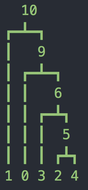
--------------------
tree 2: interval = (1143.2271080890735, 10000.0)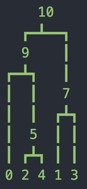
Now we have two more parameters, the length of the sequence L=10kb and the recombination rate r=2e-8 per base per generation. Now we have a sequence of trees as shown above (you might have fewer or more trees). Notice that at the top of each tree we are showing which bases follow this tree. It may seem strange that these are not whole numbers - this is because msprime uses an infinite sites model where mutations and recombination breakpoints are placed on a continuous interval (according to a Poisson process).
mu. In the example below mu=2e-8, and we also need to specify the number of sites. We can loop over the variants as shown below (so now each row is a site and each column is a sample).>>> tree_sequence = msprime.simulate(sample_size=5, Ne=1000, length=50e3, mutation_rate=2e-8)
>>> for variant in tree_sequence.variants():
... print(variant.site.id, variant.site.position, variant.alleles, variant.genotypes, sep="\t")
...
0 7658.723671920598 ('0', '1') [0 0 1 0 0]
1 22004.63021872565 ('0', '1') [0 0 1 0 1]
2 26567.67355510965 ('0', '1') [0 0 1 0 1]
3 37438.498029951006 ('0', '1') [0 0 0 0 1]In terms of the output, you should run several experiments and produce something similar to the output below (with everything after the = signs filled in). msprime acutally outputs times in generations, so you are welcome to leave them like that, or you can divide by 2N to convert to coalescent units (up to you). For all your results, experiment with n, N, L, mu, as well as K, which we'll define as the number of trials.
I would recommend running a separate series of trials for each "block" below (separated by a line of dashes). This is because you'll need slightly different parameters for each one. Overall I would recommend experimenting until your empirical results are typically within 10% of the expected values. For Tajima's d, I would recommend trying to achieve a result in the range [-10,10], i.e. something close to 0 since we'll simulate under neutrality.
For these experiments, none of them require looking at recombination, so I would leave this parameter out. If you would like to use simulated data for a final project, I would recommend including recombination to make it more realistic.
For each trial, simulate a new tree_sequence and compute the quantity of interest. Then repeat for many trials and take the average.
Here is the complete list of experiments, along with output shown below. You can add command-line arguments for the different parameters if you like, but I am also fine with them being defined in main.
Expected total branch length. As shown in the tutorial above, we can query this directly from the tree. For this part I would recommend not using mutation or recombination, just simulate a tree_sequence and take the first tree (there will only be one tree without recombination). In class we derived the expected value of the total branch length, so compute and print this value as well.
Expected time to most recent common ancestor (TMRCA). See the problem set for the expected value of this quantity. In terms of how to compute the empirical value, think about how to make use of the information in the tree. You are welcome to use any built-in functions/methods in the API Documentation.
Expected coalescent times. See the problem set for the expected values (we also talked about the results in class). The idea is to compute the time when there are n lineages, then (n-1) lineages, etc, all the way down to 2 lineages. Here I have used n=10, but this should work for any sample size. Hint: what does the order of node labels mean?
S, pi, and Tajima's d. For S and pi, there are actually built-in methods/fields to compute these quantities (see the msprime documentation). Then use S and pi to compute Tajima's d (lowercase d, we will ignore the variance). Since this data is simulated under neutrality, you should be able to get close to 0. This is the only experiment where we will need to add mutations. Also make sure to account for the number of sites, since we are considering a long region now.
$ python3 coal_sims.py
----------------------------------------------------------
Welcome to coalescent simulation experiments using msprime
----------------------------------------------------------

sample size     n = 10
population size N =
region length   L =
mutation rate  mu =
num trials      K =

----------------------------------------------------------

E[T_total]  =
avg T_total =

E[T_mrca]  =
avg T_mrca =

----------------------------------------------------------

E[T_10]  =
avg T_10 =

E[T_9]  =
avg T_9 =

E[T_8]  =
avg T_8 =

E[T_7]  =
avg T_7 =

E[T_6]  =
avg T_6 =

E[T_5]  =
avg T_5 =

E[T_4]  =
avg T_4 =

E[T_3]  =
avg T_3 =

E[T_2]  =
avg T_2 =

----------------------------------------------------------

E[S]  =
avg S =

E[pi]  =
avg pi =

E[Tajima's d]  =
avg Tajima's d =

----------------------------------------------------------
Complete the following Coalescent problems. You can either submit these on paper to the dropbox outside my office (Science Center 260) or put them on git as either a scanned image or use LaTeX. These problems are variations on some of the handout problems we didn't get to in class. Edit: here is the latex template if you want to use that for your solutions. There is also a comment about how to make your solutions in a different color.
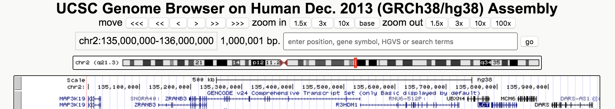
In this part we will analyze a very small fraction of the human genome:
chr2:135000000-136000000, a 1Mb (mega-base) region of chromosome 2This represents only 0.03% of the human genome! We will analyze the 1000 genomes data again. I have created the following files, separated by region or "super population".
ls -lh /home/smathieson/public/cs68/1000g/
 73M AFR_135-136Mb.chr2.vcf # African samples
 55M AMR_135-136Mb.chr2.vcf # American samples
 40M EAS_135-136Mb.chr2.vcf # East Asian samples
 57M EUR_135-136Mb.chr2.vcf # European samples
 57M SAS_135-136Mb.chr2.vcf # South Asian samples
3.8K igsr_populations.tsv   # list of populations and their "super population"
352K igsr_samples.tsv       # list of samples and their corresponding population
This VCF file format had a lot of header information ##, followed by the data, with each segregating site on one line and samples across the columns. Each individual has two chromosomes, but we will simply consider each chromosome as a separate sample. I have written the start of a VCF parser (make sure you can run it on this data). Right now the parser prints out the position and alternate allele count at every 100th SNP.
The goal of this part is to compute Tajima's d in a sliding window across this region. There are a few different ways of doing this:
Slide the window across the SNPs, taking a constant number of SNPs each time (i.e. 100). So then S is constant, and you'll need to compute pi in each window.
Slide the window across the bases, taking a constant number each time (i.e. 1000). Then compute S and pi in this window.
Try the first way, but divide by the length of the region spanned by the fixed number of SNPs (this accounts for different windows having different lengths).
Any of these ways should result in a signal in the data.
You only need to consider one population (choose any of the above). The signals in this region are present to differing extents in different populations, but all populations show some signal.
You should NOT be computing pi by looking at all pairs of samples (this will be quadratic!) Instead, look back on Handout 19 and make use of the SFS.
After you have computed Tajima's d, plot it against genomic location (see the blank template plot below).
Now look up this region on the UCSC Human Genome browser. You can copy and paste the region shown above into the search bar. You should get something like the picture below. Zoom in on the LCT gene. Do a bit of research to find out what this gene does and why it might be under selection.
Add the location of the LCT gene to your Tajima's d plot (I would recommend making it look like a horizontal line that spans the location of the gene). You can put it at any height (d=0 might be a good choice).
Make sure your plot as axis labels, a legend, and an informative title.
Finally, answer the questions in the README about your results.
![]()
Make sure to push your code often, only the final version will be submitted. The README.md file asks a few questions about human dataset. Answer these questions and make sure to push the following files.
README.mdcoal_sims.pyreal_data.pytajimas_d.png (for the real data analysis)