CS68 Lab 4: BWT and Read Alignment

Due: Wednesday, February 21 at 11:59pm

Overview

The goals of this week's lab:

Understand why we're using the BWT and FM-Index to speed up read mapping
Learn how to implement the FM-Index and verify the pattern matching results
Compare a BWT-style read aligner with a naive pattern finder
Use matplotlib to visualize the runtime results

Although you will likely have less code for this lab, I really want you to understand all the code you write and why these data structures and algorithms work for this problem. Spend some time working through the BWT and FM-Index examples from class. I have provided some examples below that use 0-based indexing, which should be easier to implement in Python. As you code and debug, really think about what is going wrong instead of just trying to match your output to mine.

Getting started and high-level goals

Find your partner and clone your lab04 git repo as usual. You should see following starter files:

README.md - questionnaire to be completed for your final submission
fm_index.py - this is where you should implement a class for the FM-Index data structure
read_mapping.py - main program that should align reads to a reference
runtime.py - a program that will perform runtime experiments and plot the results
data/ directory - sample reference genomes (strings) and reads (patterns)

You are welcome to add additional python files as long as the top-level files are the same.

Usage

read_mapping.py should take in 3 command-line arguments using the optparse library described in Lab 2:

The name of a file containing the reference sequence (FASTA) -s
The name of a file containing the file of reads (FASTA) -p
(Optional for the user) The name of a file to write the output locations of each read -o. If not specified, the output should look like the examples below.

Examples

Here are two examples we have seen in class (but now with 0-based indexing). The first computes the BWT and FM-Index for the string S=abaaba$ and then maps pattern P=aba.

$ python3 read_mapping.py -s data/reference1.fasta -p data/reads1.fasta
--------------------------------
Welcome to the BWT read-aligner!
--------------------------------

Reference sequence:
 abaaba$
Read list:
 ['aba']

BWT and FM-Index:

 i  F...L   A occ($) occ(a) occ(b)
-----------------------------------
 0  $   a   6     0      1      0
 1  a   b   5     0      1      1
 2  a   b   2     0      1      2
 3  a   a   3     0      2      2
 4  a   $   0     1      2      2
 5  b   a   4     1      3      2
 6  b   a   1     1      4      2

c M[c]
------
$   0
a   1
b   5

Mapping read: aba
    sp(  a) =   1    ep(  a) =   4
    sp( ba) =   5    ep( ba) =   6
    sp(aba) =   3    ep(aba) =   4
Start indices of aba: [3, 0]

The second example is from Handout 9, with two different patterns aligned:

$ python3 read_mapping.py -s data/reference2.fasta -p data/reads2.fasta
--------------------------------
Welcome to the BWT read-aligner!
--------------------------------

Reference sequence:
 azcdfrzccbcazctazccazbcdfzrzc$
Read list:
 ['azc', 'bc']

BWT and FM-Index:

 i  F...L   A occ($) occ(a) occ(b) occ(c) occ(d) occ(f) occ(r) occ(t) occ(z)
-----------------------------------------------------------------------------
 0  $   c  29     0      0      0      1      0      0      0      0      0
 1  a   c  19     0      0      0      2      0      0      0      0      0
 2  a   t  15     0      0      0      2      0      0      0      1      0
 3  a   $   0     1      0      0      2      0      0      0      1      0
 4  a   c  11     1      0      0      3      0      0      0      1      0
 5  b   c   9     1      0      0      4      0      0      0      1      0
 6  b   z  21     1      0      0      4      0      0      0      1      1
 7  c   z  28     1      0      0      4      0      0      0      1      2
 8  c   c  18     1      0      0      5      0      0      0      1      2
 9  c   b  10     1      0      1      5      0      0      0      1      2
10  c   c   8     1      0      1      6      0      0      0      1      2
11  c   z  17     1      0      1      6      0      0      0      1      3
12  c   z   7     1      0      1      6      0      0      0      1      4
13  c   z   2     1      0      1      6      0      0      0      1      5
14  c   b  22     1      0      2      6      0      0      0      1      5
15  c   z  13     1      0      2      6      0      0      0      1      6
16  d   c   3     1      0      2      7      0      0      0      1      6
17  d   c  23     1      0      2      8      0      0      0      1      6
18  f   d   4     1      0      2      8      1      0      0      1      6
19  f   d  24     1      0      2      8      2      0      0      1      6
20  r   z  26     1      0      2      8      2      0      0      1      7
21  r   f   5     1      0      2      8      2      1      0      1      7
22  t   c  14     1      0      2      9      2      1      0      1      7
23  z   a  20     1      1      2      9      2      1      0      1      7
24  z   r  27     1      1      2      9      2      1      1      1      7
25  z   a  16     1      2      2      9      2      1      1      1      7
26  z   r   6     1      2      2      9      2      1      2      1      7
27  z   a   1     1      3      2      9      2      1      2      1      7
28  z   a  12     1      4      2      9      2      1      2      1      7
29  z   f  25     1      4      2      9      2      2      2      1      7

c M[c]
------
$   0
a   1
b   5
c   7
d  16
f  18
r  20
t  22
z  23

Mapping read: azc
    sp(  c) =   7    ep(  c) =  15
    sp( zc) =  24    ep( zc) =  28
    sp(azc) =   2    ep(azc) =   4
Start indices of azc: [15, 0, 11]

Mapping read: bc
    sp(  c) =   7    ep(  c) =  15
    sp( bc) =   5    ep( bc) =   6
Start indices of bc: [9, 21]

In the following sections I'll discuss the different files and requirements, and give some suggestions regarding implementation.

FM-Index data structure

In the file fm_index.py, you'll implement a class called FMIndex that will compute and store the BWT, FM-Index, and suffix array data structures. You are welcome to store additional information, but at minimum you should have the following instance variables:

L: This is the BWT, the L (last) column of the sorted cyclic permutations (i.e. rotations) of S (the original string).
F: This is the F (first) column of the sorted cyclic permutations of S. Note that this is not part of the FM-Index, but we will keep it for printing and debugging.
A: This is the suffix array A, where A[i] is the index of F[i] in the original string S.
M: This is a table where M[c] is the first index of character c in the F column.
occ: This is the occurrence table, where occ(c,i) is the number of times character c occurs in L[1...i] (inclusive).

Here are a few recommendations and options for implementing these data structures:

Have your constructor take in the original string S (including a $ at the end). Your constructor should build all these data structure, but it might be useful to have helper functions along the way.
When sorting the rotations, you are welcome to use the built-in Python sorting functions. You can either sort in place (a example below), or not (b example below). You can also sort based on a more complex function of the values. For example, the special list below is sorted according to the second entry of each value (which is why it ends up getting sorted by the ints).

>>> a = [5,3,1,7,2]
>>> a.sort()
>>> a
[1, 2, 3, 5, 7]
>>>
>>> b = [5,3,1,7,2]
>>> b_sorted = sorted(b)
>>> b_sorted
[1, 2, 3, 5, 7]
>>> b
[5, 3, 1, 7, 2]
>>>
>>> special = [["three",3], ["one",1], ["two",2]]
>>> special.sort(key=lambda x: x[1])
>>> special
[['one', 1], ['two', 2], ['three', 3]]

Either during or after sorting the rotations, you'll need to retain the index of each F[i] in the original string so you can form the suffix array A.
Although M is the smallest part of the FM-Index, it might take a bit of work to figure out the best way to store this information. You'll need to be able to look up the value given a character c. You'll also need to be able to look up the value for the character alphabetically after c.
For the occurrence table, I would recommend a numpy array, but this is up to you.

In terms of methods for your class, you should have at least the following:

CONSTRUCTOR: The constructor which takes in string S and computes the FM-Index and other data structures as described above.
MAP READ: A method for mapping a read (pattern) after the FM-Index is computed. This method should take in a read (string) and return a list of indices in the original string where the pattern begins. It is fine for this list to be empty, indicating that the given pattern never occurs in the input string. Use the recursive formulas developed in class on Wednesday for this part (it is completely fine to implement this method recursively or iteratively). I would recommend that this method also include a boolean parameter verbose for specifying whether or not additional output should be printed (as shown above). If this flag is False then nothing is printed, which will be helpful for large files.
REVERSE: A method for reversing the BWT to obtain the original string. You don't need to include this method in the output, but you should run it as part of your testing and validation (described below).
STR: A __str__ method that returns a nice string representation of the FM-Index and related data structures. It should look roughly like the example outputs above, but you are welcome to include more information or display it in a different but helpful way.

Note: if you are interested in pursuing a non-class option for this part (to avoid class overhead or experiment with reduced memory-footprint) talk to me first, but it should be fine in principle.

Testing your FMIndex class

You should have testing code in your FMIndex class (or as a separate file). In addition to testing your data structures, you should test the pattern indices of some examples by using the built-in Python index method. Consider the example below, where ab occurs twice in S. Use this idea to develop a method for returning all start indices of a given pattern, so you can compare this with your results using BWT. At the end of the lab you'll compare the runtime of this naive index method with the runtime of the BWT method.

>>> S = "dcabccdbab"
>>> S.index("ab")
2
>>> S.index("ab",3) # start searching again right after 2
8

Read Mapping

In the file read_mapping.py, you should have your main program that parses the two input files (FASTA format), computes the BWT and FM-Index, and displays this information to the user. There are two different ways this program should work:

If an output file is NOT specified, display the type of output shown above ("verbose" mode). You can check whether or not the file was specified by testing if opts.out_filename is equal to None.
If an output file IS specified, print minimal output as shown below (since the BWT and FM-Index can be very large). Then instead of printing the read locations, write them to the output file in the format shown below.

$ python3 read_mapping.py -s data/ecoli_ref_small.fasta -p data/ecoli_reads_small.fasta -o ecoli_locations.txt
--------------------------------
Welcome to the BWT read-aligner!
--------------------------------

Reference sequence length G:
 11941
Number of reads n:
 2000

Finished BWT and FM-Index
Finished mapping reads

Here is the output file in this example: ecoli_locations.txt. Note that here I sorted the indices first so if you're comparing your results with the built-in index you can use diff.

Runtime Analysis

The last part of the assignment to analyze and visualize the runtime of this FM-Index approach vs. a naive pattern finding method. This part should be in runtime.py. Requirements for the runtime analysis:

Your runtime analysis should be conducted on the files:
- /home/smathieson/public/cs68/ecoli_uti89.fasta (reference)
- /home/smathieson/public/cs68/ecoli_reads.fasta (reads)
It is not necessary to use the entire reference genome (this will likely run out of memory!) Start by experimenting with small fractions of the reference and small fractions of the reads.
There are two options for your runtime analysis. The first option is to plot the runtime as a function of the number of reads. The second option is to plot the runtime as a function of the length of the reference genome.
We will compare our runtime to the runtime of the naive built-in index method discussed above. So for each read, your method and the index method should return exactly the same list of indices. The idea is to compare how long this process takes for each method.
You are welcome to use any method to time the results, but I would recommend using the time library: time. Store time.time() (in seconds) before the code you want to time, and then repeat after it's finished. If you choose to plot runtime as a function of the number of reads, you will be analyzing some of the same reads multiple times; that's okay.
Should you include the time to compute the BWT and FM-Index? That's up to you. On one hand it is pre-processing that is done once and can be stored indefinitely. On the other hand, it still is part of the runtime of read mapping. Either way is fine for this lab.
Before you start, develop a hypothesis about the results you expect. What is the time complexity of each method? What constants are important? (see README.md)
Don't write the results to a file, we are just going to time the actual mapping process.
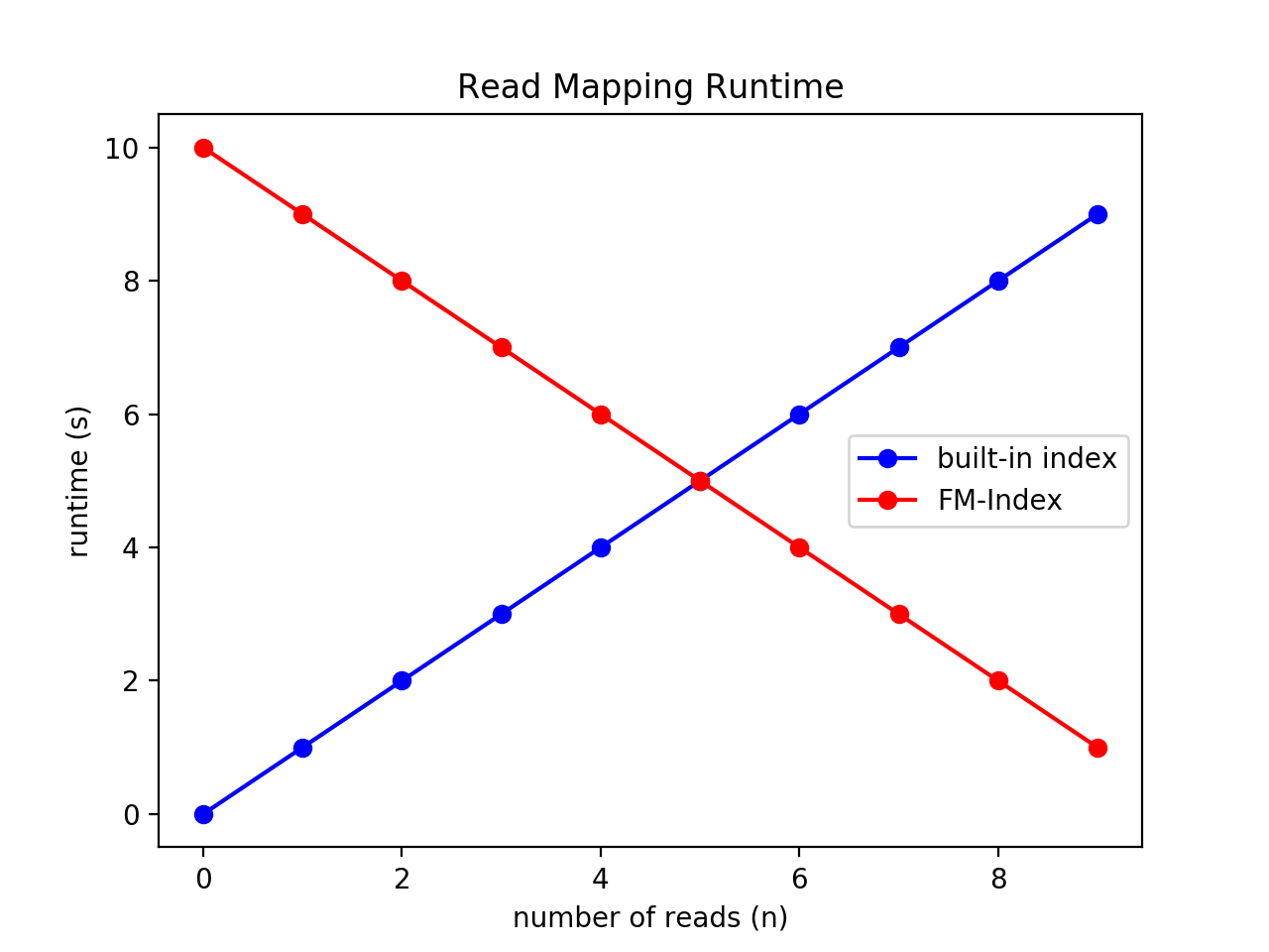
Finally, plot your results using matplotlib. Here is an example below (similar to the example in Lab 2). These lines are completely made up and not realistic, they are just to provide an example. If your results take a long time to run, you are welcome to write them to a file, and then read them in separately to create your plot. Either way, the file that creates the plot should be runtime.py.
To save this plot, you can either click the save ("disk") button from plt.show(), or use plt.savefig("runtime_plot.png",format="png"). You can also use pdf, etc. Make sure to push your plot and any associated files necessary for creating it.

>>> import matplotlib.pyplot as plt
>>> x = range(10)
>>> y1 = x
>>> y2 = [10-val for val in x]
>>> plt.plot(x,y1,'bo-')
>>> plt.plot(x,y2,'ro-')
>>> plt.title("Read Mapping Runtime")
>>> plt.xlabel("number of reads (n)")
>>> plt.ylabel("runtime (s)")
>>> plt.legend(["built-in index","FM-Index"])
>>> plt.show()

Additional requirements

Your program should follow good design practices - effective top-down design, modularity, function/method headers, file headers, and comments.
You may submit as many additional files as you wish.
Practice defensive programming; e.g., did the user provide enough arguments on the command line? Do the files exist? You do not need to check if the contents are correct.
Do not interact with the user for your program - if an incorrect filename is given, simply exit the program with a message; do not prompt for a new file.
Clean up any debugging print statements.

Extensions (optional)

Storing the entire occurrence table takes a lot of memory. In reality, modern read-mappers store only a subset of entries (say every 100th row) of the occurrence table (as well as the suffix array). In this extension, modify your code to keep every kth row of just the occurrence table. This creates a hybrid approach where we'll need to scan the BWT (L column) a bit to find out how many desired characters are between these checkpoints.

We are again at a time/space tradeoff. By storing less information, we need to recompute some values on the fly, but the space savings are usually worth it in this case. Experiment with how many rows you keep and how much this affect the time and space. To figure out the memory footprint of an object, you can use:

import sys
sys.getsizeof(<obj>)

The second extension involved mismatches (errors or population-level sequence variation). This is open-ended, and I would recommend investigating the Bowtie paper posted in the reading for inspiration. The idea is that instead of just keeping track of the true "next" character, we keep try different options for this character that represent mismatches. By only allowing a few mismatches we keep the number of back-tracing paths small, but we also allow variation to be captured which is extremely important. Extending BWT style aligners to mismatches is the innovation that allowed them to be used on next-generation sequencing data.

Analysis and Submitting your work

Make sure to push your code often, only the final version will be submitted. The README.md file asks a few questions about your runtime analysis. Answer these questions and make sure to push the following files. Do not push long files of read location results.

README.md
fm_index.py
read_mapping.py
runtime.py
runtime_plot.png (it is fine to push multiple plots but remove out-dated ones)